Routine MoK(alpha) data collection

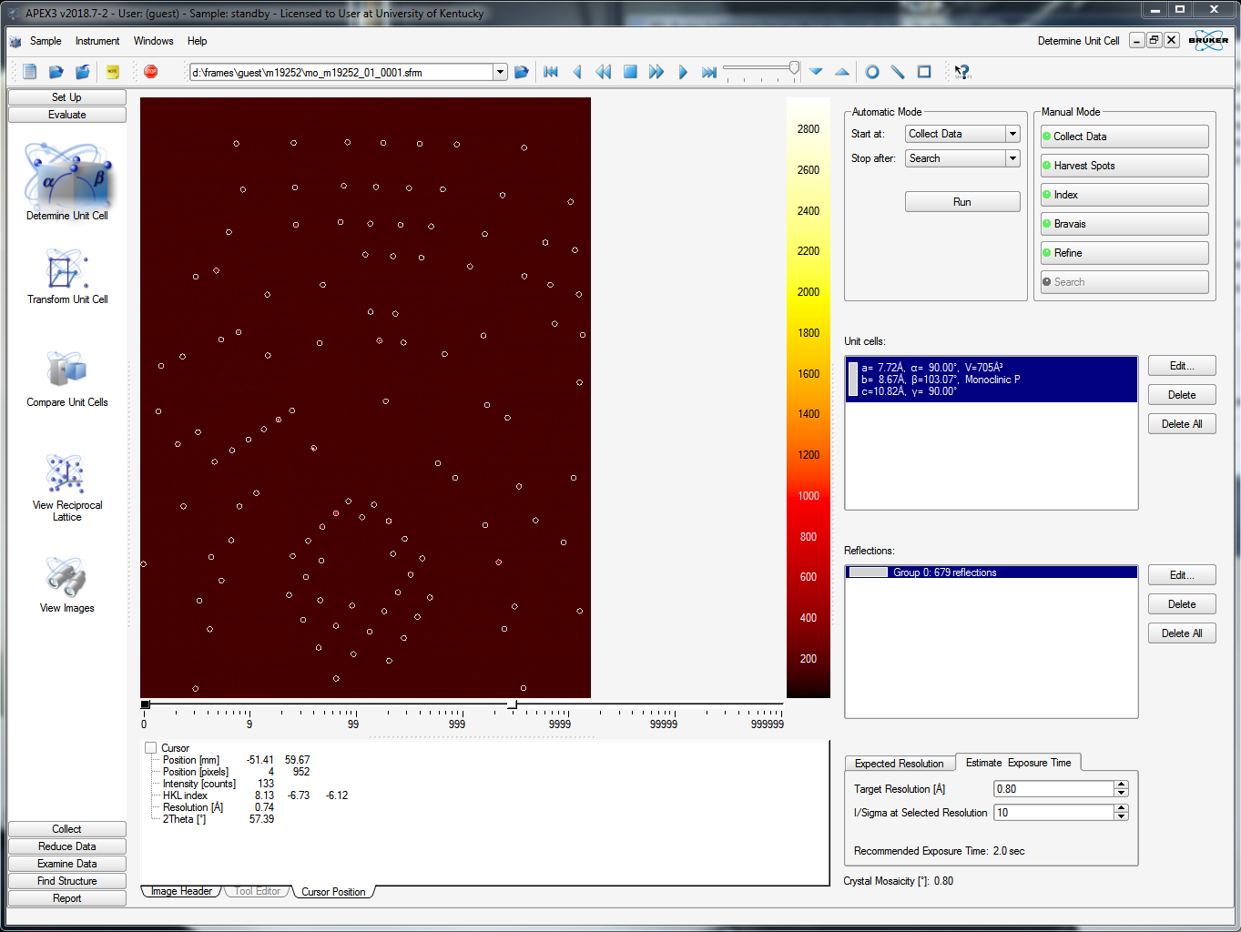
9) Index the crystal using the fast scan

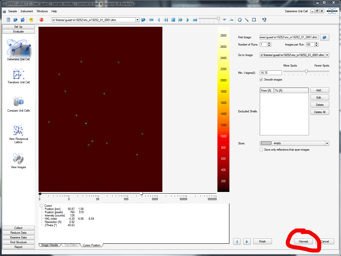
Once the fast scan is running and you've watched a few frames whiz by on the APEX3 window, you should try to index the crystal. On the left-hand-side vertical menu, select "Evaluate" and then "Determine Unit cell". The default APEX3 window for this functionality is shown below. In the upper right of the window, find the "Number of Runs:" box - it should be set to 1. That's your fast scan! Next to it there's a box for "Images per Run:". The default entry here is 20, but you should set it to the number of fast-scan frames that have already been collected. The more frames the better. In the image below it has been set to 60, which is plenty. Go ahead and click "Harvest" down in the bottom right.

$harvest diffraction spots$

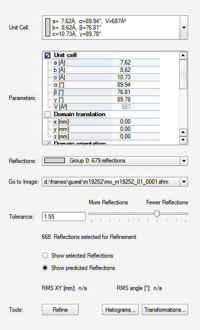
APEX3 scans through the specified number of images and finds the diffraction maxima in each image according to threshold criteria (see the slider in the above picture, upper right - about half way is a reasonable starting point, it should be obvious what it does). It saves the x and y coordinates and the rotation angle (cylindrical coordinates!). In this case it tells you it found 679 reflections, like this:

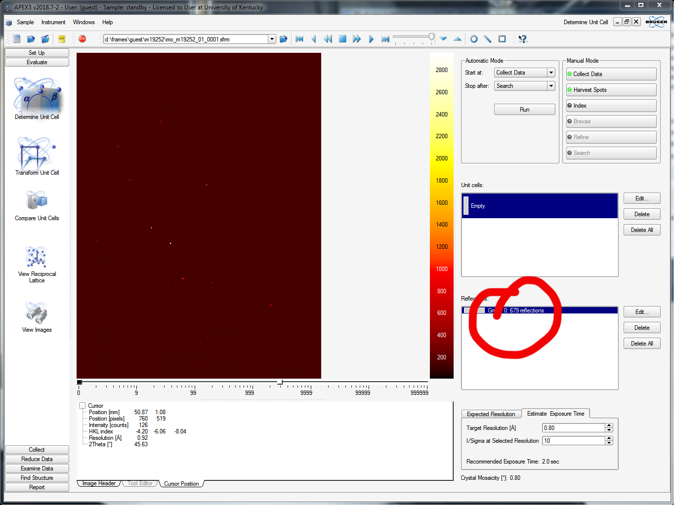
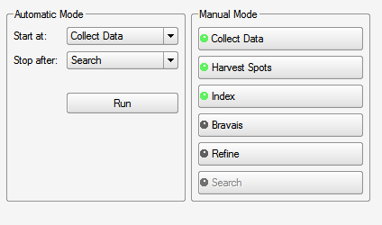
When you click "Index" you get the following:

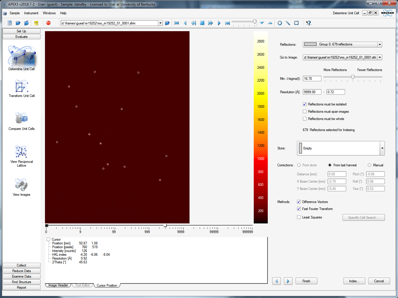
This allows you to fiddle a bit more with the reflections that will be used to index. On the first pass, there's little point in changing anything, so go ahead and click the "Index" button on the lower right. It tries two different algorithms: "difference vectors" and "fast Fourier transform". When both methods work (a good sign!) you get something like this snippet from the APEX3 window:

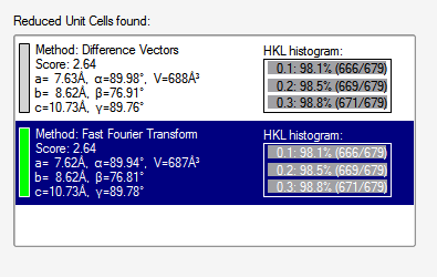
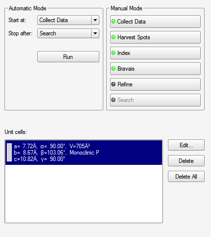
Sometimes one routine works while the other fails. Occasionally, if the crystal has some nasty problem, both will fail. There is a third indexing option, but it is beyond the scope of this exercise. Since both methods gave the same result, we could accept either. Sometimes they look a bit different but are equivalent, e.g., the β angle for monoclinic could be given as either acute or obtuse. When you accept one of the results, you get something like this (snippet):

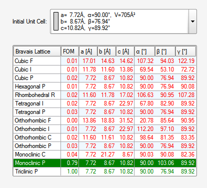
At this point you could click "Refine" to optimize the result a bit prior to transforming the unit cell to a standard setting and checking for higher symmetry. The goal is to find the standard Bravais lattice. You guessed it, click "Bravais" ...

... which brings up this table:

The easiest way to interpret this table is to read the "FOM" column upwards (FOM = figure of merit) and look for the place where the FOM drops to a low value. Usually, the highest entry with a comparatively large FOM is correct. The program selects its best guess, which is often (but not always!) correct. In the above picture, it should be obvious that the Bravais lattice is primitive monoclinic. Notice also that it has transformed β to be >90°, which is the conventional setting for monoclinic. It will also set α and γ to exactly 90°, as shown below.

Indexing gives both the unit cell parameters and a mathematical description of the crystal orientation in matrix form. The "Refine" button optimizes the cell and the "orientation matrix". You can get a good idea of how well the assigned unit cell fits with the diffraction spot positions by clicking on the "Histograms" button.

Here, it should be pretty obvious that the cell is assigned correctly. The x and y distributions are very narrow, and h,k,l indices are integers. The width of the rotation angle distribution is limited by the angular frame width, which for our fast scan was set to 1°. For this particular crystal, everything is close to perfect.

We now have the crystal properly indexed along with a good mathematical model for the crystal orientation. We should, therefore, be able to predict where any reflection (hkl) appears on any of the diffraction images. The right mouse button lets you see predicted positions, as in the above picture.

Your job now is to decide whether to collect a full dataset. If you have the CSD handy, you could check the unit cell to see if it is known. With a good fast scan, you probably have sufficient data to quickly solve the structure. If it is your intended product, or something even better, then you will need to go ahead and set up for a full data collection. Since this tutorial is intended to show how to collect good data, we'll just assume we have a quality crystal. In which case, the final step is to set up a good data collection strategy. To do this, proceed to step 10.