8) Inspect the diffraction pattern using a fast scan
To inspect the diffraction quality, we'll use APEX3. It is probably running on the main monitor, but if not, start it from its icon. It might take a moment or two to start up. When it comes up, under "Sample" choose "New ...".
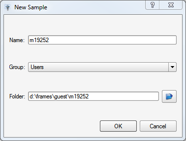
In the "New Sample" box, type a new structure code. For MoKα on the UK D8 Venture, type m19252, where "m" signifies "MoKα", "19" is the year, and "252" is the numerical sequence number, which you can figure out from previous entries in the log book. For CuKα data, use "c" in place of "m", and find its sequence number (likely a few pages back in the log book).
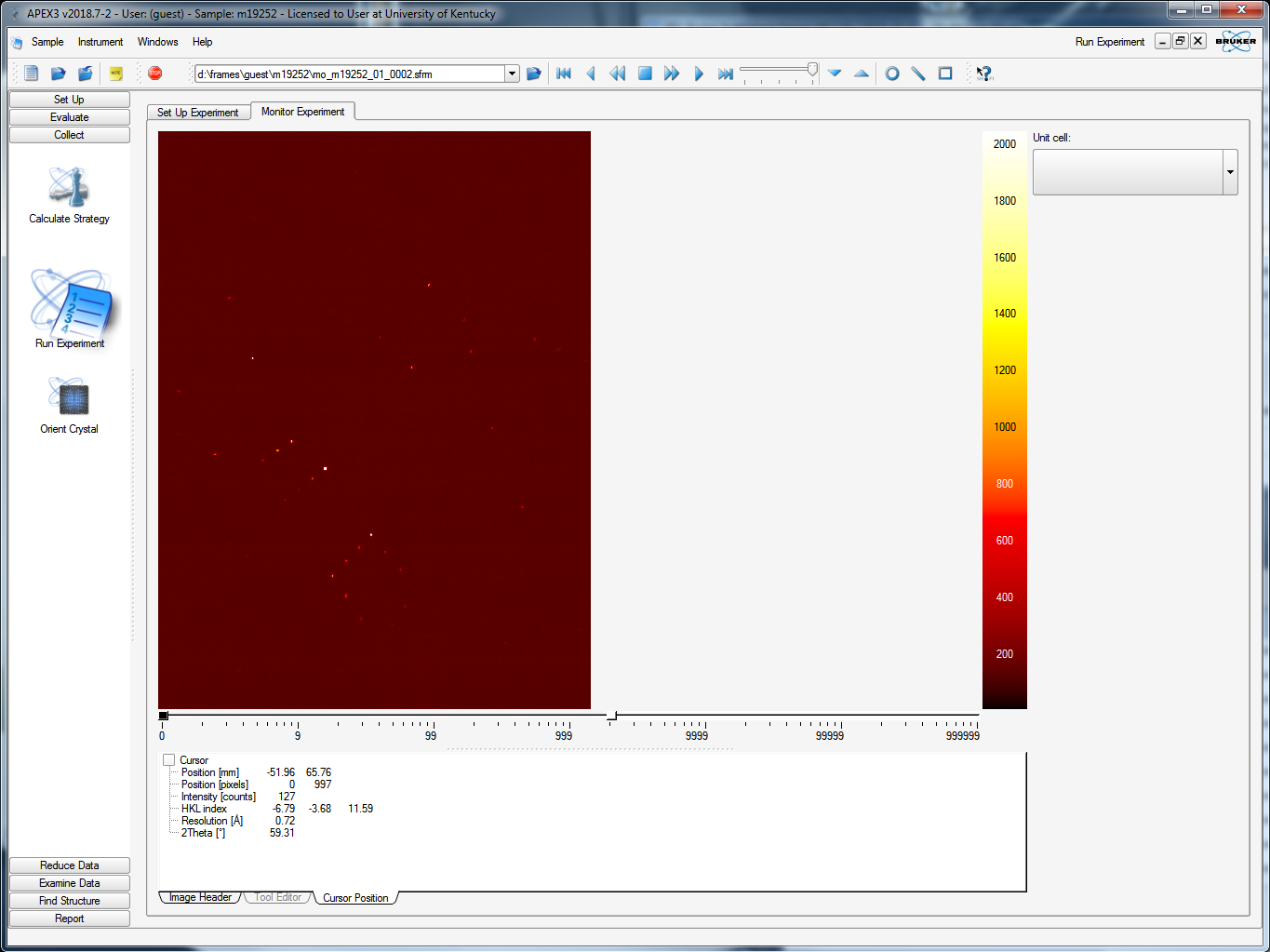
Under "Describe sample", enter as much information as you can. Also remember to add an entry in the log book. You can see the sort of information to write by looking at other log entries. Notes are essential in science for many reasons, amongst which, someone might have to figure out what you were doing ten, or more years later! Back to the job: select "Collect" from the left-hand-side menu, and click "Run Experiment", which brings up the data collection spreadsheet, like this:
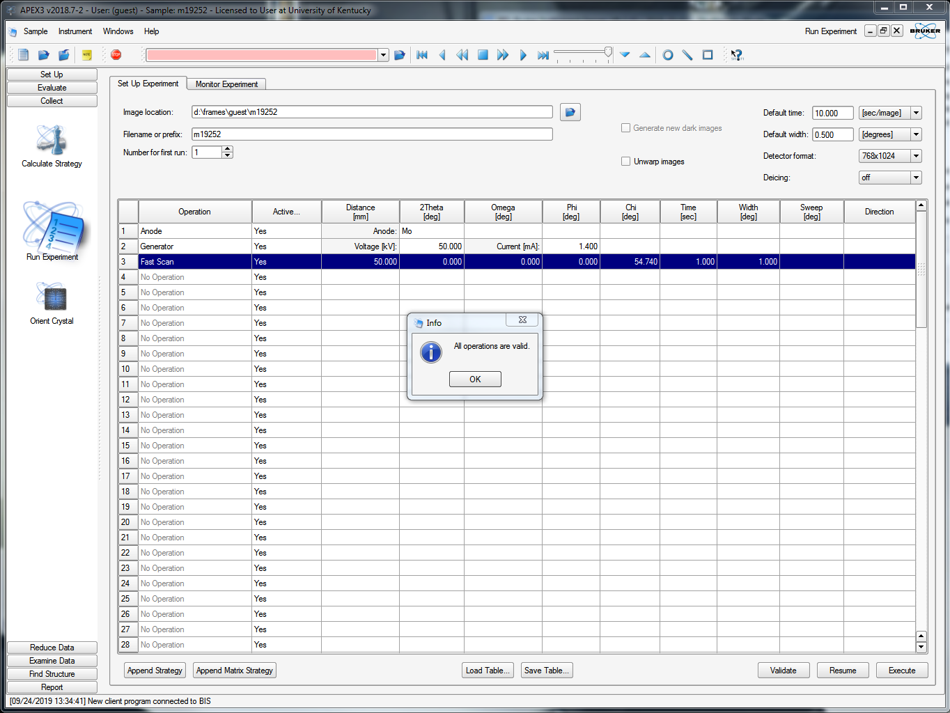
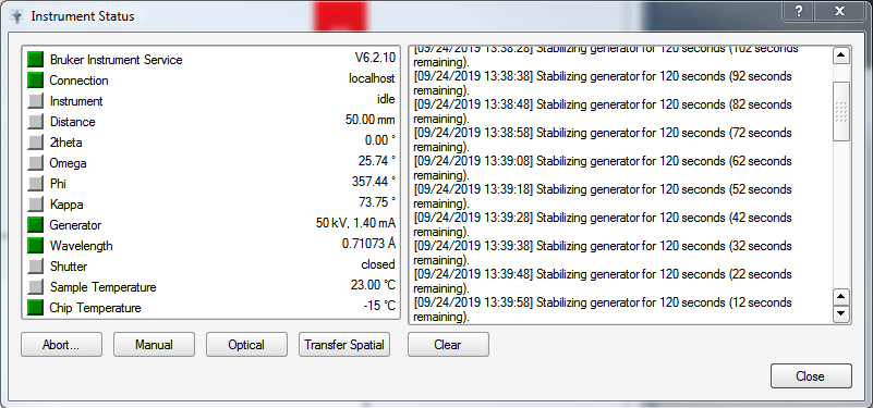
Ensure that the Anode is set to Mo. Beneath that on line 2, select "Generator" and make sure it is set to 50kV and 1.4mA. On the next line select "Fast Scan", as in the above picture. Click "Validate" in the lower right. Assuming all is ok, click "Execute". If the generator was already at full power, it proceeds to collect. If it has to crank the power up it will do that and then wait for a few tens of seconds to stabilize the generator prior to opening the shutter. You can watch the stabilization progress (amongst other things) in the Instrument Status window (on the top menu, click "Instrument", then "Show status"). It looks like this:
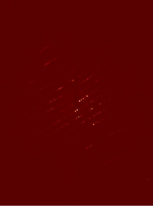
When the generator is stable, the goniometer moves to the start of the fast scan, opens the shutter, and starts collecting. If it looks good, as in the picture below ...
... then let it keep running. If it is bad, then you should stop it and either slow it down (e.g., 2s, 4s, 10s frames etc.) or perhaps go back to the microscope to select a new crystal.
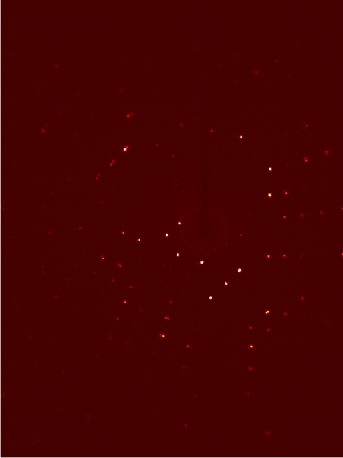
The criteria that constitute acceptable diffraction depend on the sample at hand, analysis of which is beyond the scope of this exercise. The diffraction pattern below is a 1° frame from a high-quality sucrose crystal. All visible diffraction spots are sharp and single, with no streaks or split reflections.
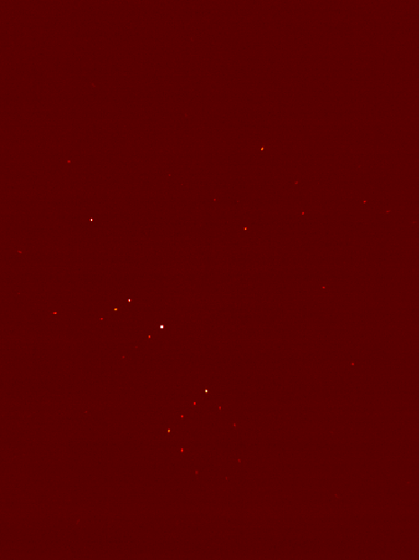
Obviously, for some other crystal, even of the same material, the spots would be in different places. For larger unit cells there'll be more diffraction spots and vice versa. If you have a cracked crystal, it might look more like this:
Notice that some of the spots are split. A cracked crystal has more than one piece, and the pieces will be misaligned. Since each piece has its own reciprocal lattice, there'll be two (or more) diffraction patterns. The misalignment of the reciprocal lattices (visible in the diffraction images) is due to misalignment of cracked fragments. If that's all you have then you might have to live with it. If you have better crystals available, it's best to switch now.
Other crystal problems manifest themselves in different ways. With experience you will see all manner of lousy diffraction patterns. The following image ...