10) Collect a full, complete dataset
To collect a full, high-quality dataset, the diffractometer needs to be told where to scan in order to sample enough of reciprocal space. To accomplish this, we must figure out a strategy. On the left-hand-side of the APEX3 window, click "Collect" and then select "Calculate Strategy". You should get a window that resembles the following:
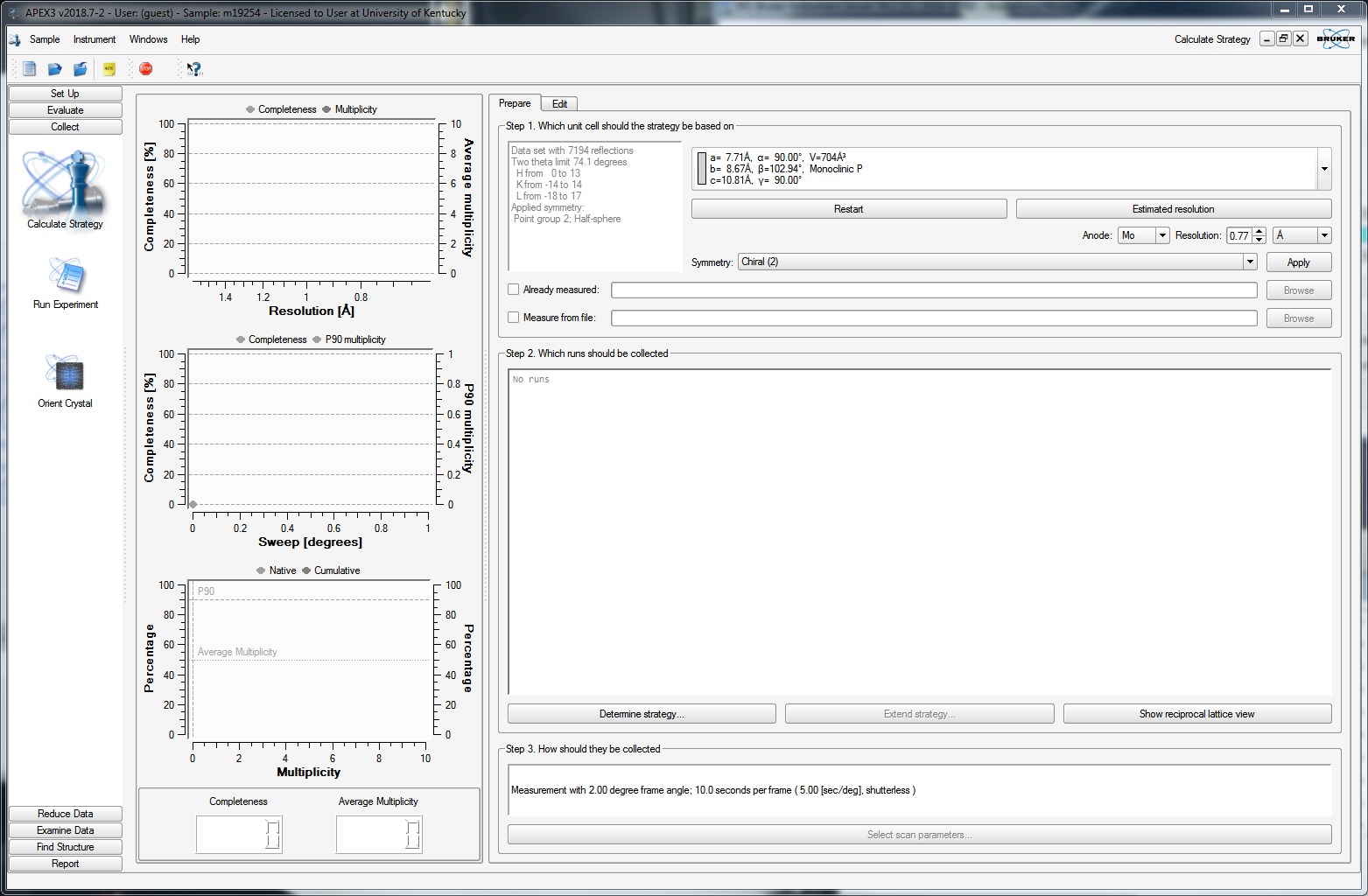
The strategy generator already knows the Bravais lattice, which in large part defines how much of reciprocal space to scan, but you get to set a few additional criteria. In our case here (sucrose), we know the structure is chiral, so you can leave that alone. Bear in mind, however, that with a light-atom compound using MoKα X-rays, there'll be essentially zero anomalous signal, so you could justify (in this case) unsetting the "chiral" criterion. If you don't understand what that means, then seek professional help. You can set the maximum resolution - here it is set to 0.77Å. You could go to a bit higher resolution (smaller value), but there's little point in going to lower resolution. If you remember, 0.77Å with Mo is about 55° in 2θ, which is equivalent to 180° 2θ with Cu X-rays (i.e., the absolute upper limit for Cu). Higher resolution will give you more unique data, but for this routine structure, it won't add much of any particular value. When you're ready, click "Determine Strategy", which gives you the following:
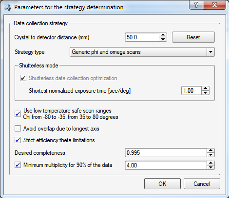
Here you get to set a few more things. For the crystal-to-detector distance, 50mm is a good distance unless you have a cell edge that is more than about 25Å. A useful rule-of-thumb for MoKα X-rays if there's a cell edge >25Å, is to set the distance (in mm) to twice the longest cell edge (in Å). For example, if you had a unit cell with a 30Å cell edge, you'd set the distance to 60mm. On this instrument you should check the "low temperature safe ...", which will prevent the χ angle getting too small or too large. The reasons for this were explained way back in part 3. We also set the minimum multiplicity to about 4, which ought to be fine for sucrose. For heavily absorbing crystals, a bit more (say 5 or 6) will give greater multiplicity of observations (aka redundancy), which will help in defining an empirical absorption correction during data processing. After clicking "OK", the program will calculate a strategy. Sometimes the computer seems to get unresponsive, but it usually recovers, and presents you with:
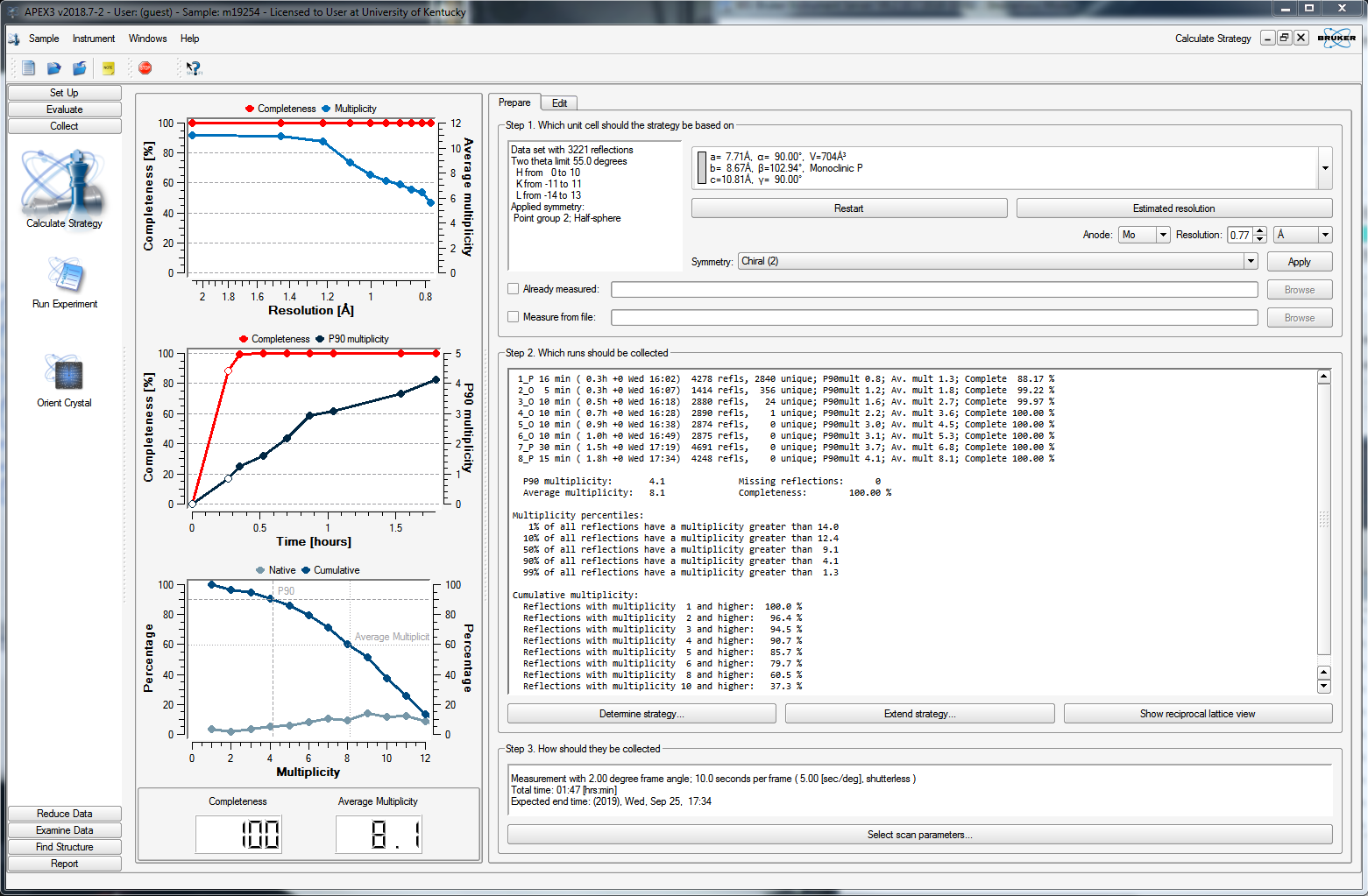
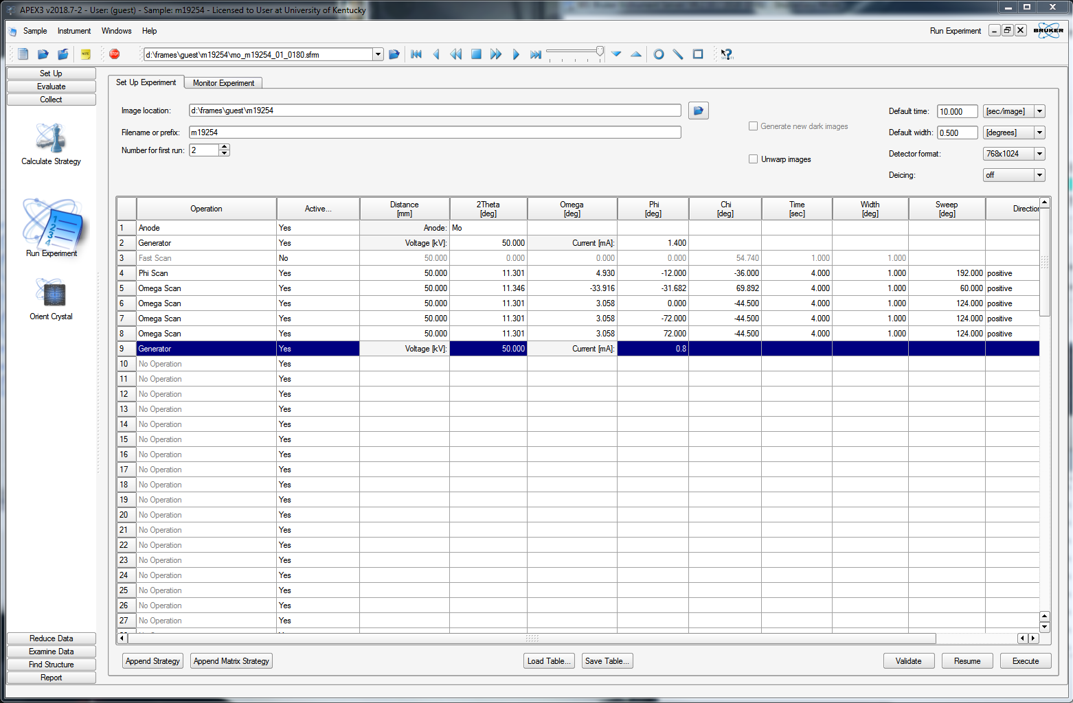
For this case (above), it predicts 100% completeness with a multiplicity of 8.1 in eight scans. It looks as though the data are 100% complete after just four scans, while the multiplicity will be 4.5 after five scans. You could therefore truncate the strategy at four or five scans. To do that, click the edit tab to get a list of the scans, like this:
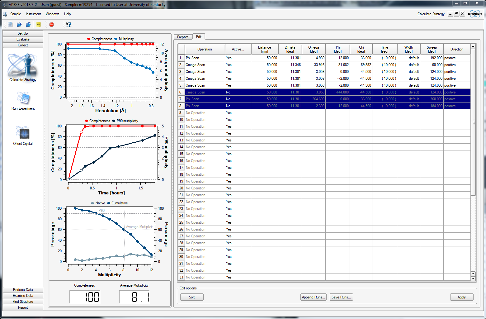
You can delete any superfluous scans or set their "Active" status to "No", as in the above. When you click back on the "Prepare" tab, it will recalculate some of the statistics, as shown below.
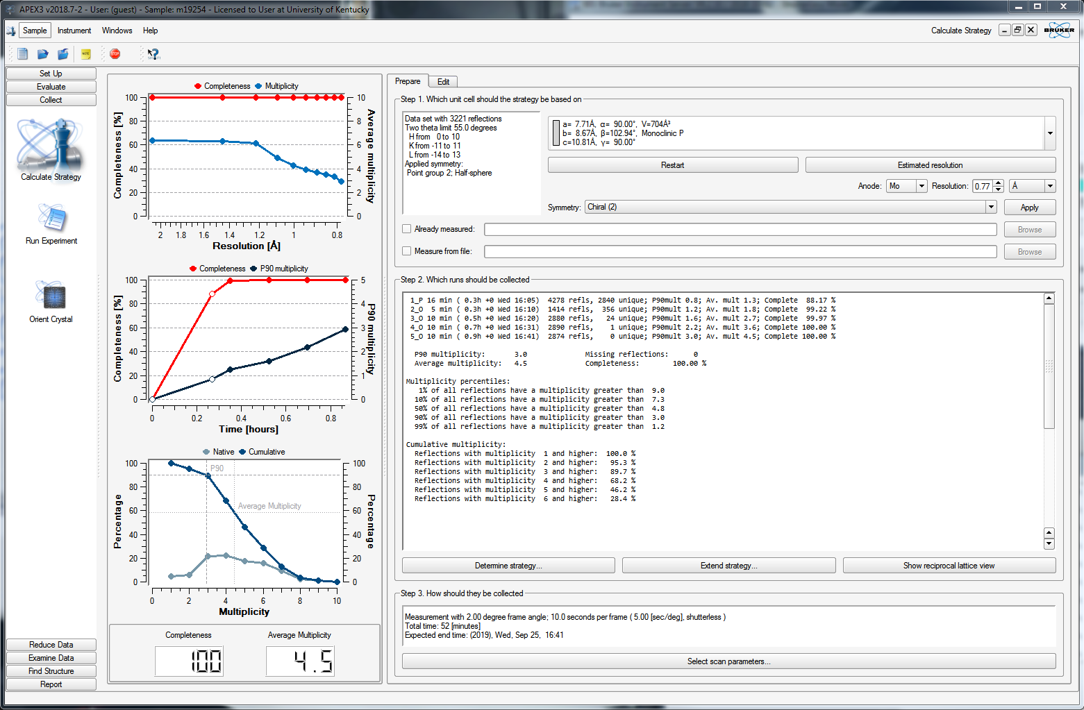
At this point, you need to set an exposure time for each frame. On clicking the "Select scan parameters ..." button on the bottom of the APEX3 window, you get this:
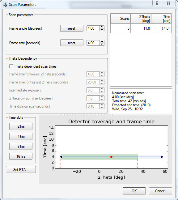
There are a few options here, but we'll keep it simple. You should enter a frame time that gives good intensities at higher resolution. You should also be wary of overloading the detector, which is all too easy with a good crystal. Remember the fast scan? over in the BIS window, there should be a record of how many (if any) frames in the fast scan had "topped" intensities. If there are a lot, then it is probably best to redo the fast scan, but even faster. There are far more detailed diagnostics for frame-by-frame overload analysis, but they're way beyond the scope of this tutorial. The fast scan(s) is(are) used to replace overloaded intensities in your main scans. If your initial fast scan was free of overloads, then a reasonable exposure time for your main scans might be between 4 and 10 times as long as the fast scan. Here we set it to 4, then click "OK".