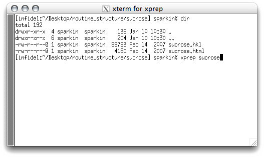
To start XPREP, simply type 'xprep sucrose' at the prompt and hit the
<return> key. If your '*.hkl' file is not named 'sucrose', then you need
to use that filename instead of 'sucrose'. The program is smart enough to look
for a file with the '.hkl' extension. This will give you something like this:
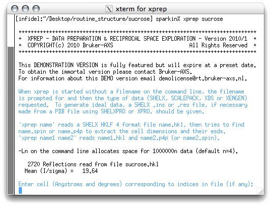
To enter the cell dimensions you simply type them in. As stated above, the best
estimates of the cell dimensions available from data collected on the kappaCCD are
contained in the nreport.html file, which is a summary of data collection,
scaling and merging statistics. Since it is an ordinary html file, it can be
read with a web browser or with a text editor. To open it with (say) firefox, then
type 'firefox filename.html' (again, substitute the proper filename here!). It
looks something like this:
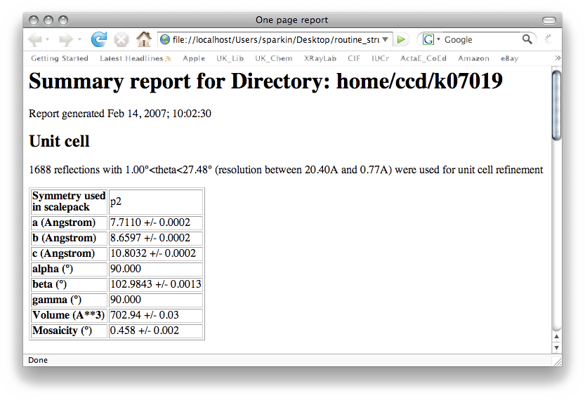
You may notice the filename given at the top of this nreport.html (k07019) is different
from the filename we are using (sucrose). Renaming to 'sucrose' was just for the sake
of convenience. The k07019 name follows the convention used in the X-ray lab. at UK
(k = kappaCCD, 07 = the year 2007, 019 = the 19th data collection done that year). You
can of course use whatever filename you like, but it helps with bookkeeping if you
follow some sort of convention.
It is always best practice to keep good notes. This is especially true for novices, so write these numbers down in your notebook! Also make note of the uncertainties that are associated with each of the cell dimensions. You will need these later (vide infra). In any event, type the cell dimensions into XPREP, all on one line and separated by spaces like this:
It is always best practice to keep good notes. This is especially true for novices, so write these numbers down in your notebook! Also make note of the uncertainties that are associated with each of the cell dimensions. You will need these later (vide infra). In any event, type the cell dimensions into XPREP, all on one line and separated by spaces like this:
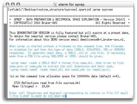
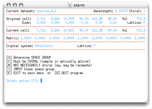
When you hit <return> you will get the following:
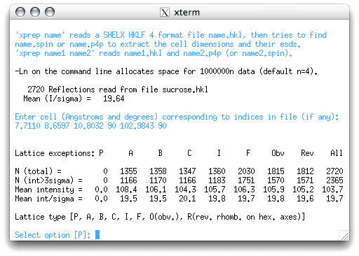
One of the great things about XPREP is that it usually makes sensible choices.
Nevertheless, it helps to know what is going on. The table in the window above allows you
to tell the program whether the crystal has a primitive or a centered unit
cell. If you don't know what that means, consult your notes or an introductory textbook.
So, how to read this table? Notice there is a column for P (primitive), as well as columns for various centering conditions (A,B,C etc.). Below these labels there are numbers that tell you how often a particular criterion is violated. Since it is always possible to fit a primitive lattice to a set of regularly-repeating points in 3D space, there should always be a bunch of zeroes in the P column. The other columns have non-zero numbers in them. If the unit cell was centered, then it would be apparent from the numbers in these columns. For example, if the lattice was really I-centered (the I means body centered, and is from the German innenzentriert), then the intensity found for any reciprocal lattice point with an odd number for h+k+l, would be negligible. In the table this would give small numbers in the I column for the bottom two rows.
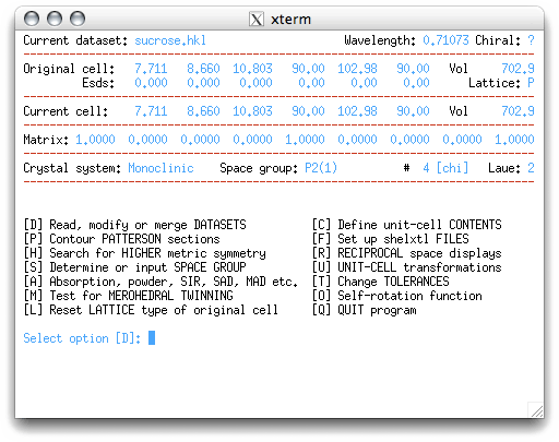
XPREP usually makes the right choice, and gives its best guess in square brackets. Since the cell is indeed primitive, all you have to do is hit <return>. This brings up the main XPREP menu:
So, how to read this table? Notice there is a column for P (primitive), as well as columns for various centering conditions (A,B,C etc.). Below these labels there are numbers that tell you how often a particular criterion is violated. Since it is always possible to fit a primitive lattice to a set of regularly-repeating points in 3D space, there should always be a bunch of zeroes in the P column. The other columns have non-zero numbers in them. If the unit cell was centered, then it would be apparent from the numbers in these columns. For example, if the lattice was really I-centered (the I means body centered, and is from the German innenzentriert), then the intensity found for any reciprocal lattice point with an odd number for h+k+l, would be negligible. In the table this would give small numbers in the I column for the bottom two rows.
XPREP usually makes the right choice, and gives its best guess in square brackets. Since the cell is indeed primitive, all you have to do is hit <return>. This brings up the main XPREP menu:
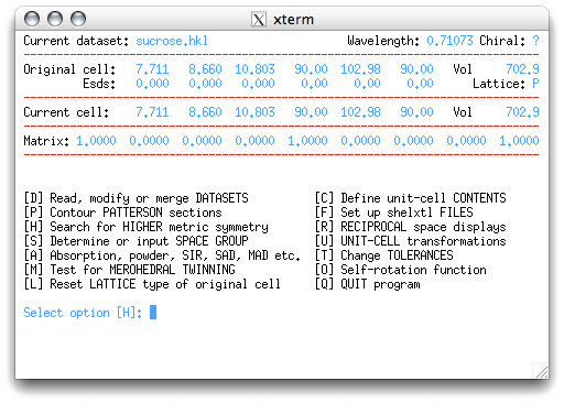
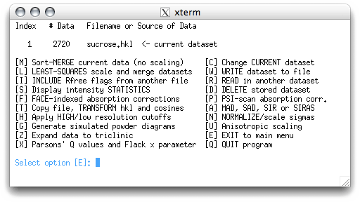
In this example, we will only use a small subset of the tools available in XPREP.
If you feel the need to try the other features, go ahead. Some of these will be used in
later tutorials for more difficult structures.
XPREP suggests the option H, which will search for a higher-symmetry cell. When you hit <return>, the program responds like this:
XPREP suggests the option H, which will search for a higher-symmetry cell. When you hit <return>, the program responds like this:
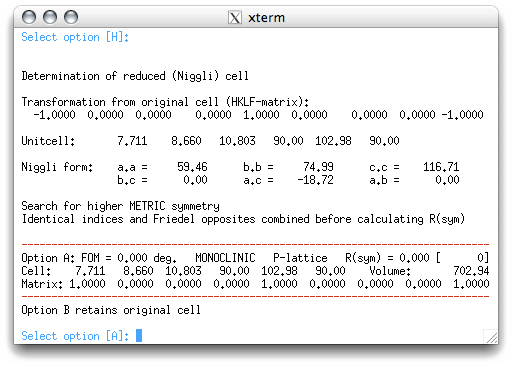
In this example, the program suggests a cell that is identical to the one you typed in.
It also gives a second option that retains the original cell. In this case, options A
and B are the same. More complicated structures might give a few different possibilities
for you to consider. In this case, however, the program is not able to find a higher
symmetry cell, so we accept the default value by hitting <return>. This sends us
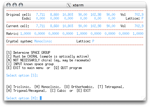
back to the main menu, which now suggests the "S" option for space group determination:
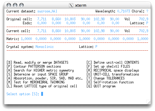
Do the obvious thing, hit <return> to get this:
If you know the space group already, you could enter 'I' at the prompt. Since we know
that sucrose is chiral, we could enter that here, but let's make the program do all the
work! Go ahead and enter 'S', as suggested by XPREP:
To proceed, the program needs to know the crystal system. It can usually figure this out
from the metrics of the cell, but there are cases where it can be deceived, e.g. for
a monoclinic crystal with β=90° it will suggest orthorhombic. Here it makes the
correct choice of monoclinic, so accept the default value of 'M' by hitting <return>.
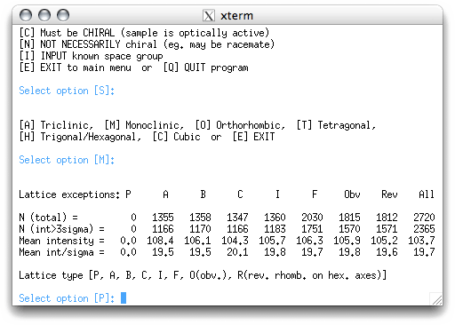
Here the program gives you a chance to revise your choice of centering, but it is
unusual that you'd want to change this. In this case, you know it is primitive, so
accept 'P' by hitting <return>, which gives:
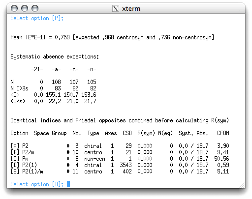
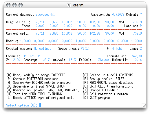
Here we get three blocks of information:
The mean |E*E-1| statistic gives information on whether the structure is likely to be centrosymmetric or non-centrosymmetric. All it does is to compare the value calculated for the dataset (0.759) with a theoretical value for centrosymmetric (0.968) and non-centrosymmetric (0.736) intensity distributions. Here it is clear that the sucrose data are non-centrosymmetric, and this makes sense. Sucrose molecules are chiral, and at least with naturally occuring sucrose there is only one enantiomer. This means that it has to be non-centrosymmetric. This statistic must be treated with caution because it can be misleading. Examples of such problems usually involve data from twinned crystals, pseudo-symmetric crystals, non-centrosymmetric crystals that happen to have centrosymmetric distributions of heavy atoms etc. None of those problems concern us here because the |E*E-1| value is reasonable.
The next block tells us about the presence of screw axes (written as -21- in the table column heading) and glide planes (written as -a-, -c-, -n-). The table is laid out in much the same way as the table used to decide on the presence of lattice centering. In this example there are no violations for the 21 screw axis, but plenty of violations for the a,c,n glide planes. Again, this makes complete sense. Since natural sucrose has just one enantiomer, there can't possibly be any glide planes in the crystal structure because glide planes include a mirror operation. Note: depending on how the data reduction was performed, there may have been non-zero numbers in the 21 column. This would happen if the systematically absent reflections were left in the dataset during merging and scaling. If you don't know what this means, you may want to find out. Either way, it should be apparent that there is a 21 screw axis in this structure.
XPREP uses all the information gathered so far to try to ascertain the space group. There are usually a few suggestions along with a bunch of information that enable you to make an informed choice. Probably the most useful statistic here is the CFOM (combined figure-of-merit), which is usually smallest for the correct space group. In this case, XPREP suggests option 'D', P2(1), which is just the SHELX way of writing P21. Accept this by hitting <return>.
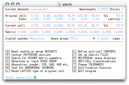
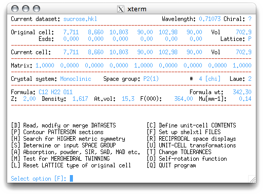
We're back at the main menu, but with the 'D' option recommended as the next step. In
this tutorial we will simply hit the <return> key through these screens, but a
brief explanation of each will be given:
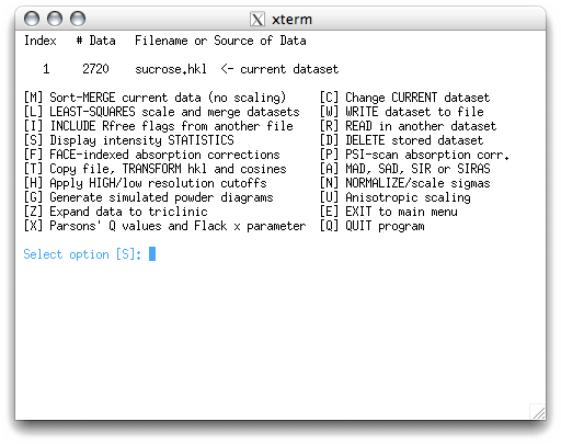
This is a separate sub-menu. The program wants to show you some intensity statistics,
hit <return>.
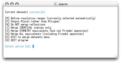
Merging and intensity statistics depend on whether symmetry equivalents have been merged
or not. Feel free to try the different options. If you try the suggested 'A' option you
get the following:
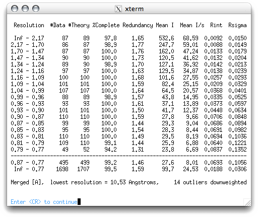
As you can see, there's a lot of information. The table splits the data into resolution
shells with roughly the same number of reflections in each. The Rint
column gives a measure of whether symmetry equivalents have the same intensity. Notice
that in the higher resolution shells (lower down the table), the Rint
values get larger. The mean intensity and mean I/sigma tend to get smaller at higher
resolution, while the Rsigma get larger. These variations with resolution
happen because diffraction intensities tend to be weaker, and therefore more susceptible
to noise, at higher resolution. As a general rule, the data are usable so long as the
mean I/σ for a shell is >2 and the Rint < 0.3, but there is some leeway.
There is little point in including very high-resolution reflections if all they contain
is noise, so you may occasionally have to truncate the high-resolution limit a bit
(seek help if you are unsure). In any event, this sucrose data is strong throughout
the whole resolution range.
On hitting <return> we get the following.
On hitting <return> we get the following.
This sends us back to the main menu:
The 'C' menu item allows us to enter the molecular formula:
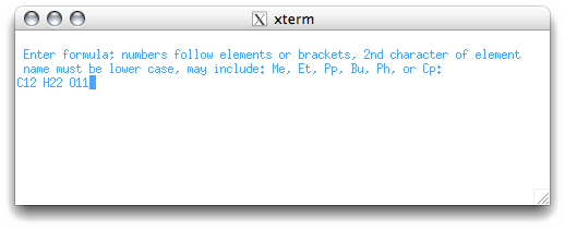
It is not absolutely necessary to know the formula, but it does help. If you don't know
it, you can make up something plausible based on what the starting materials were, but
remember to correct it later! When a formula is entered you get a chance to change some
other stuff, as follows.
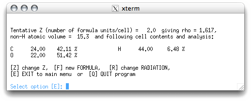
The Z value is the number of formula units in the unit cell. The program estimates Z
based on the formula and the unit cell volume. If you have the formula correct, this is
usually a good estimate. On returning to the main menu, you get this:
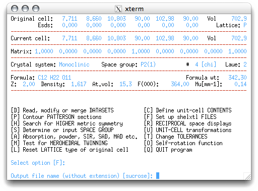
The next menu item selected is 'F', which sets up the files to be used by SHELXS,
the structure determination program. On hitting <return>, you get to choose the
filename for your instructions ('.ins') file:
For a routine structure it is ok to keep the same file name, but in some circumstances
you may need to change it. This could happen if you had to re-index your data for any
reason, e.g. if you found a higher symmetry cell. Here we choose the default
'sucrose', by hitting <return>. You get a choice of whether to use SHELXS
(most common) or SHELXD (mainly for difficult cases). There is now a third
option, SHELXT, which will work with files created for either SHELXS or
SHELXD.
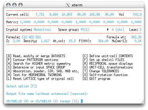
For this example, choose 'S' for SHELXS, to get:
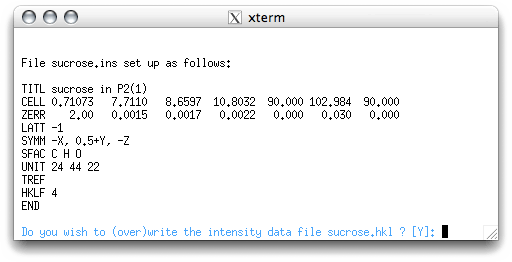
XPREP gives you a listing of the instructions file ('sucrose.ins'),
and the option of writing (or overwriting) the data file. You may recognize some of
the numbers given here. The numbers on the CELL line are the wavelength of the X-rays
in ångstrom units, followed by the cell dimensions. On the ZERR line below CELL, the
numbers are Z (i.e., the number of formula units) followed by standard uncertainties
(SU values) for each of the cell parameters. Unfortunately for kappaCCD data, the SUs
written by XPREP are incorrect. The proper values are given in the nreport.html
file, which means you will have to manually edit the '.ins' file to enter the proper
values (you'll do this next). The rest of the commands in the '.ins' file will be
explained in the next section of this tutorial. You are now ready to quit XPREP
and solve the structure, so hit <return>.
This sends you back to the command line of the terminal window. If you want to see what
files XPREP has created, type 'dir' and hit <return> (note: the
'dir' command is used in the UK X-ray lab. as a shorthand alias for the unix
command 'ls -l', so it may not be present on unix systems outside this X-ray
lab.).
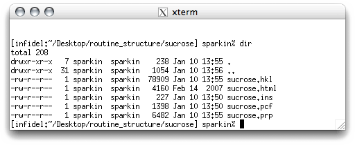
There should be three new files, sucrose.ins, sucrose.pcf,
sucrose.prp. As stated above, sucrose.ins contains instructions for the
structure solving program, SHELXS. The file sucrose.prp contains a listing
of all the stuff that was written to the screen by XPREP, which can be useful for
diagnostic purposes. The file sucrose.pcf contains a bunch of information written
in CIF format. Note: for data collected
on the kappaCCD, not all of the information in the .pcf file is correct, but you
do not need to worry about that.
Part 1: Setting up instructions - XPREP
Part 2: Structure solution - SHELXS
Part 3: Molecule editing - XP
Part 4: Structure refinement - SHELXL
Part 5: Ellipsoid and packing plots - XP
Part 6: The Crystallographic Information File - CIF
Part 2: Structure solution - SHELXS
Part 3: Molecule editing - XP
Part 4: Structure refinement - SHELXL
Part 5: Ellipsoid and packing plots - XP
Part 6: The Crystallographic Information File - CIF
Return to the first page of this tutorial
Return to the main Tutorials page or to the main X-Ray Lab page
Return to the main Tutorials page or to the main X-Ray Lab page