Large b in SHELXL  WGHT

4/4: A SADABS remedy for large b in WGHT

We’ll use a recent gold-containing complex ‘STG-2’ (Gilpatrick et al., 2024) that happened to give particularly weird looking WGHT parameters.

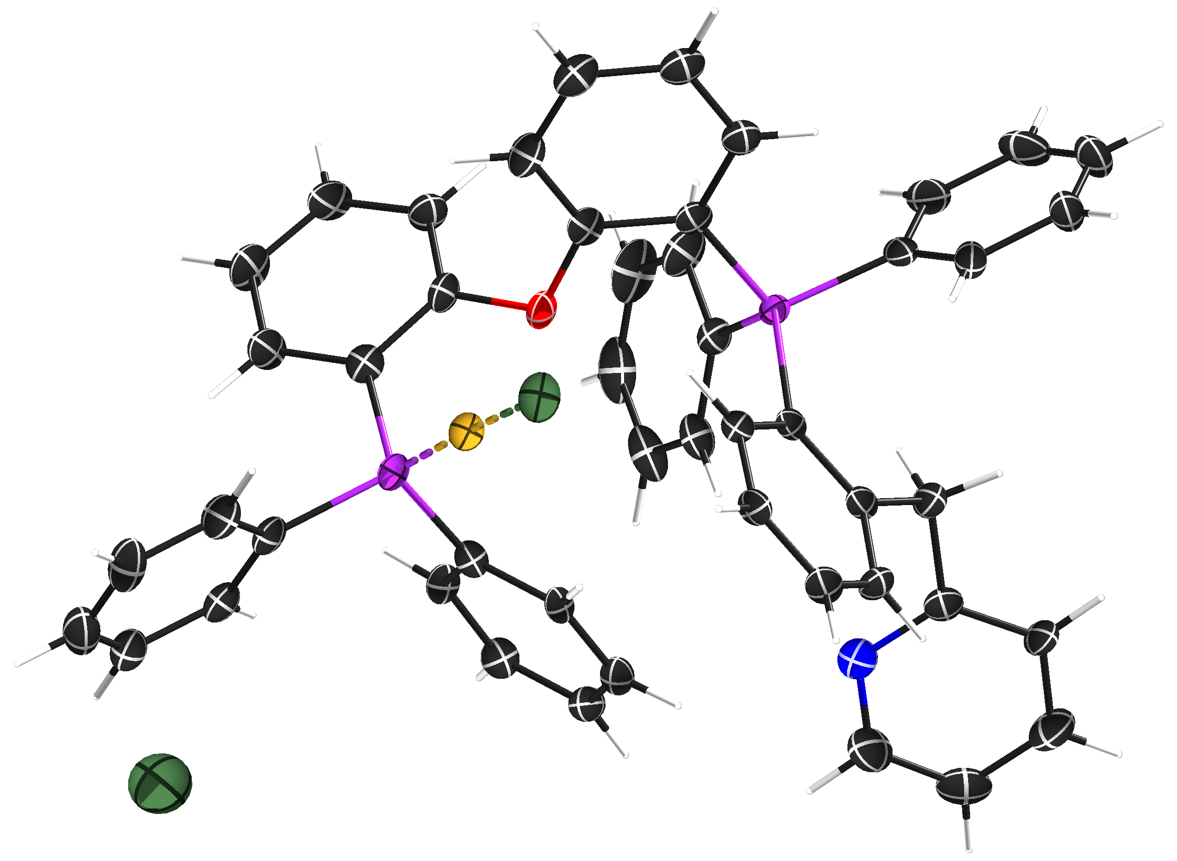
Fig. 2. An ellipsoid plot of gold complex STG-2.

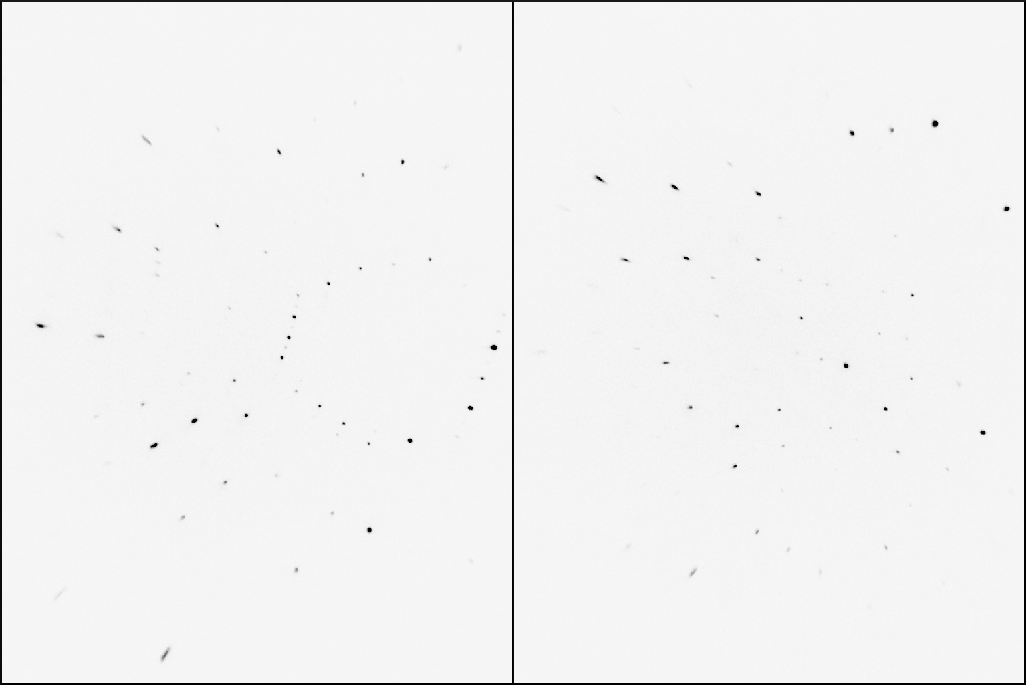
This was a CuKα dataset, which is not ideal for a gold compound (our MoKα optics were broken at the time), but diffraction images all looked fairly good (see Fig. 3) and gave no obvious indication of problems. The published STG-2 made use of SQUEEZE (Spek, 2015) but was otherwise well behaved, so the unusual WGHT parameters were a surprise; related structures were not similarly affected. The *.raw, *.hkl, *.fab, and *.res files are available here.

Fig. 3 Data frames from STG-2 in two different regions of reciprocal space. Nothing seems to be amiss.

Use of default values forced by the APEX gui version of SADABS gave K in the range 0.817-0.984 and a refined g of 0.0447, which in turn gave the following WGHT parameters for a fully refined model:

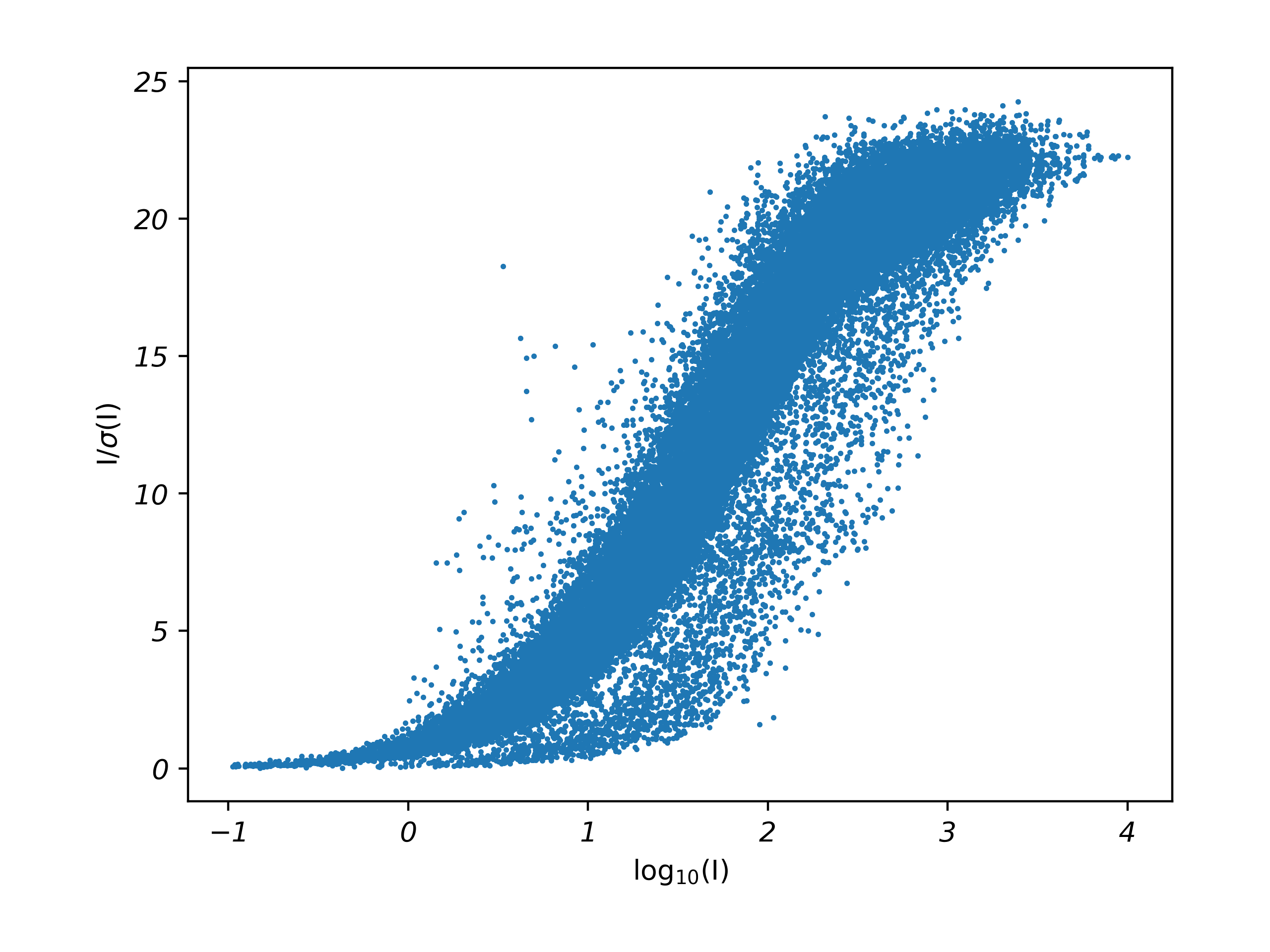
This default SADABS run gave the Diederichs plot shown in Fig. 4, indicating a limiting I/σ(I) of 22.4. For context, values quoted by Krause et al. (2015) range between 16.4 and 82.5, and the authors suggest a value of ~30 being good for synchrotron data. Thus, the overall data quality for STG-2 seems reasonable for a routine structure.

Fig. 4. Diederichs plot for STG-2 from a default SADABS run. Note the abundance of points at the upper right [high I/σ(I)] of the scatterplot.

After a bit of experimentation, setting sm = 3.4 as the 12^th parameter on the HKLF command subsequently led to:

The a parameter is still zero, but b takes on a much more normal-looking value. Let’s see if we can achieve something similar using command-line SADABS.

For an initial test we'll try fixed K = 3 and g = 0.0447. It is likely going to take some iteration to optimize so we’ll give each trial a separate filename (e.g., ‘fix-K3-g’), which should help us to keep track of progress. For the first trial, we’ll track the full screen output of the SADABS run as we go and give brief explanations where necessary. The input raw data filename ‘c24009’ is just the sequence number in the UKy X-ray lab logbook assigned to STG-2 when the data were collected. The next few text boxes show the screen output of the command-line SADABS run (highlights indicate changes from defaults).

Choose ‘expert mode’ to access to all facilities within SADABS and change the name of the log file.

Above, we enter the raw data file that was created by SAINT during integration.

All entries in the above terminal snippet are defaults ...

Again, all defaults (some repetitive lines deleted) ...

Here we specify option 11, fix K = 3, and g = 0.0447, which results in the following:

Notice that the I/s(lim) value is just the reciprocal of g, i.e., 22.4 = 1/0.0447.

Aside: Here we also change the μR of an ‘equivalent sphere’ in order to better approximate the 2θ-dependent component of the absorption surface. The recommendation given by Krause et al. (2015) for a crystal of size 0.3 x 0.2 x 0.1 mm with μR = 10 mm^-1 is to use an effective sphere radius of 0.07 mm, which upweights the smallest crystal dimension by ~5.5 times, viz.

Therefore,

This approximation works surprisingly well in most cases. As shown in the above box, for STG-2 the crystal was 0.20 x 0.15 x 0.07 mm and had μ = 8.42 mm^-1, giving μR = 0.41 mm^-1. As a result, one might consider using a more aggressive set of spherical harmonics for the absorption correction than the default, but that is fodder for another tutorial.

We now have a newly written dataset ‘fix-K3-g.hkl’ and its attendant log (.abs) file. We can rename a copy of the previously refined model (for STG-2 we’ll also need the .fab file since it used SQUEEZE ) and iterate the refinement until the WGHT parameters converge. This can be done manually, but is easily automated using ShelXle  (Hübschle et al., 2011) and presumably other programs (it is also possible to script using bash or python).

Such a test gave the following:

We’re clearly going in the right direction. The a parameter looks reasonable, and b is much reduced, so let’s try K = 4. There’s no need to explicitly present all the SADABS output again, simply repeat the above steps but use K = 4, g = 0.0447, and use the filename ‘fix-K4-g’, which gives:

So, we’re still heading in the right direction. After running a few more trials (again, this could be automated with python /pexpect or bash /expect ) with K increasing by 0.1 each time, the results tabulate, as follows:

It looks as though K of about 4.3 in SADABS produces sensible-looking weights and any further increases in K are overkill. A Diederichs plot for this treatment is shown in Fig. 5.

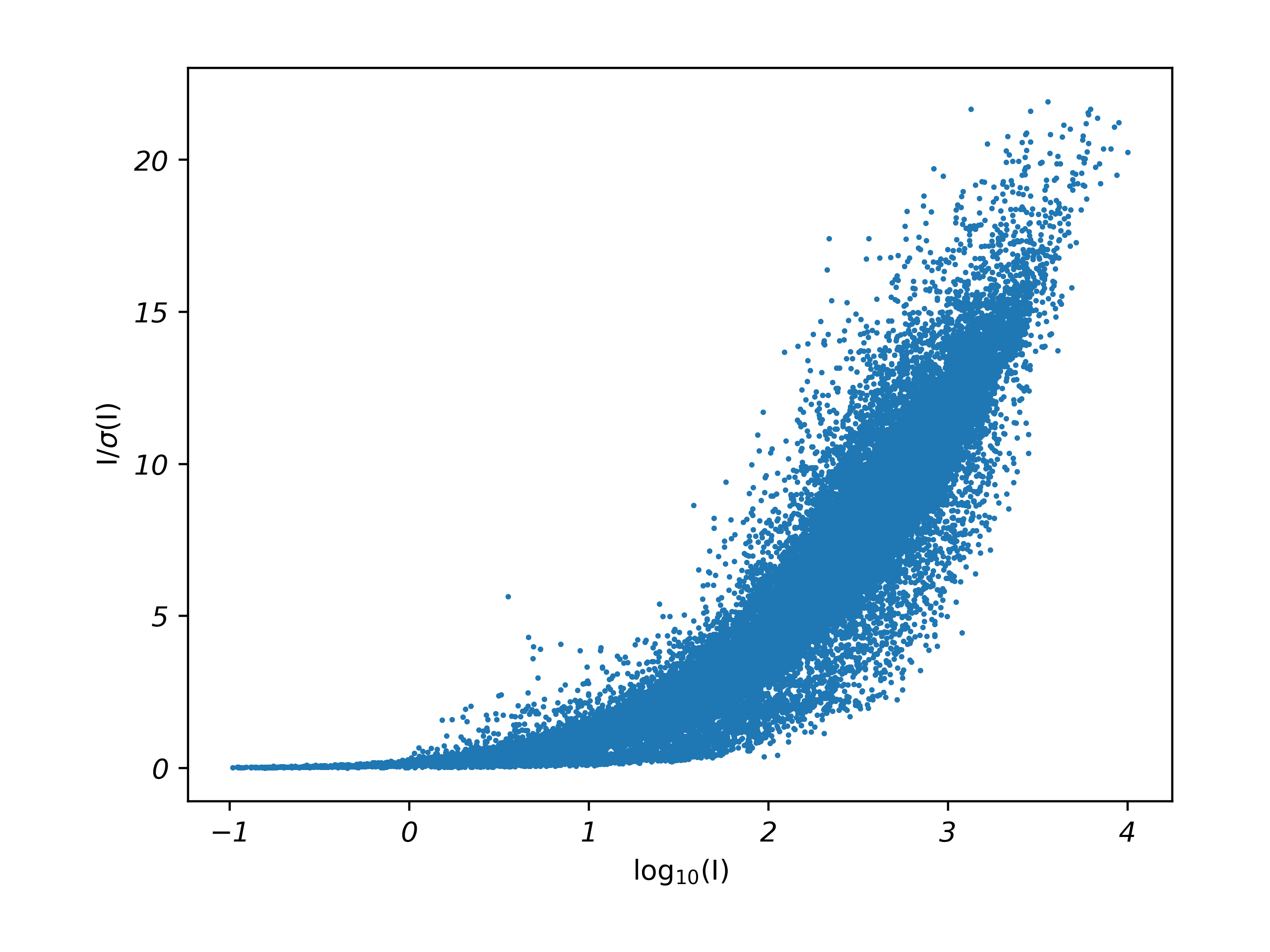
Fig. 5. Diederichs plot for STG-2 from a SADABS run using K = 4.3 and g = 0.0447.

Note that the height of the scatter plot in Fig. 5 matches the default run in Fig. 4, but many of the points are shifted to lower I/σ(I), leaving the plot a little sparse in the upper right. That’s to be expected, as the σ(F_o²) had been previously diagnosed as underestimated.

The high b problem is thus 'fixed' for STG-2, while preserving most other details, including the 'flatness' of the analysis of variance (see *.lst file) and the overall I/σ(limit). This was an extreme case; few large-b WGHT problems will require such a big K value in SADABS. Something like a K of 1.1 — 1.3 is more typical.

Aside: It's important to note, however, that none of this makes much difference to the resulting structure model. Does any of it matter ? I don't know. My own view is that it might be preferable to leave it all as is so that everyone has the same information, not hidden in a SADABS log file. I've always been a bit leery of the 'forcing the goof = 1' notion. If there's a bona fide statistical basis for that, it's alien to me, and (apparently) much of the statistics community. The goodness-of-fit should be 1 for distributions drawn from the same population. Observed and calculated F² don't fulfill that criterion, especially if the spherical-scattering-factor approximation is used (that's most structures). It's silly to think that they should.

The last bit of that comes from my notes as a grad. student in 1992 when we first got a beta version of SHELXL-92 at UC Davis. They are basically a paraphrase of Håkon Hope's comments in a group meeting. (Message to students: keep copies of your notes.)