Electron density and Fourier theory
Electron density in a crystal is tri-periodic. It can be calculated using the following
equation:
in which, the summations are over positive and negative indices, and
x, y, z — real-space coordinates
V — unit cell volume
h, k, l — reflection indices
F — structure factor
For an introductory exercise, all of the important concepts can be addressed in one dimension. To use a real molecule in the analogy, however, we need to generalize a bit and make the problem mono-periodic. [n.b. 'mono-periodic' and 'one-dimensional' are not synonymous, but are often used interchangeably. It is usually easy to tell what is meant from the context.]
In a mono-periodic 'crystal' with repeat distance 'a', the above equation for electron density reduces to:
Using Euler's formula, e iφ = cos(φ ) - i sin(φ ), we can expand this into cosine and sine terms:
The electron density equation is thus a sum of different frequency sinusoids, i.e., a Fourier series.
Consider a hypothetical mono-periodic crystal of carbon dioxide, a linear centrosymmetric molecule. A ball-and-stick representation of CO2 looks like this:

A 1–D plot of its electron density looks qualitatively something like this:
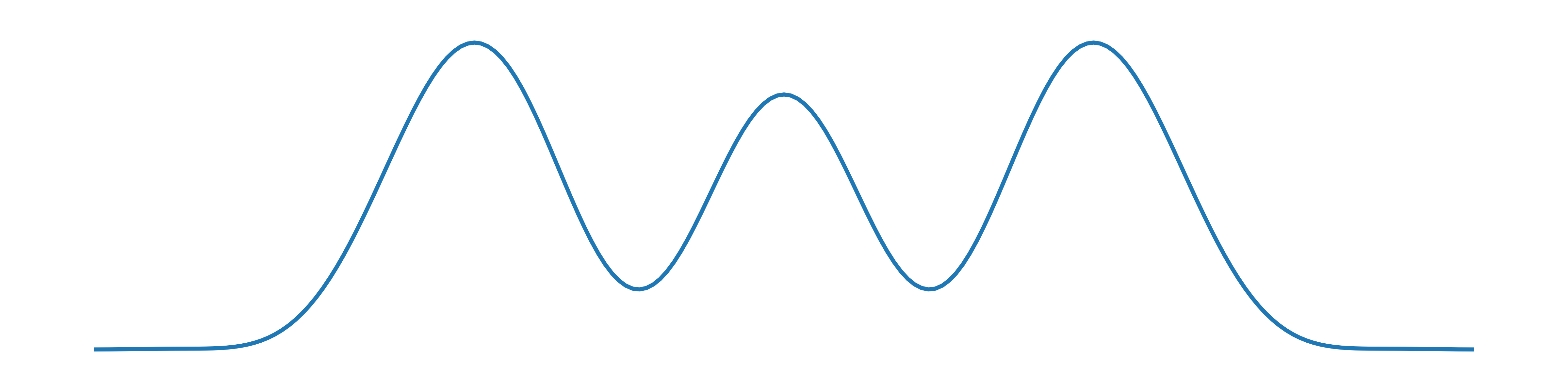
The oxygen atoms have larger peaks than carbon because oxygen has eight electrons, while carbon only has six. The electron density drops down to a flat baseline on either side but in the bonds it is non-zero.
In such a made-up crystal, the molecules are arranged in a line. Five in a row might look like this:

For which, the electron density 'wave' would be:

Since it is periodic, we can model it using the above Fourier summation. Assuming a repeat distance of 5.00Å and one molecule per 'unit cell', the electron density looks like this:
The area under the curve must equal the number of electrons in the unit cell. For a single CO2 molecule, that's 22e–. A properly scaled plot of electron density is thus quantitative. The question is, what superposition of waves will approximate this curve ?
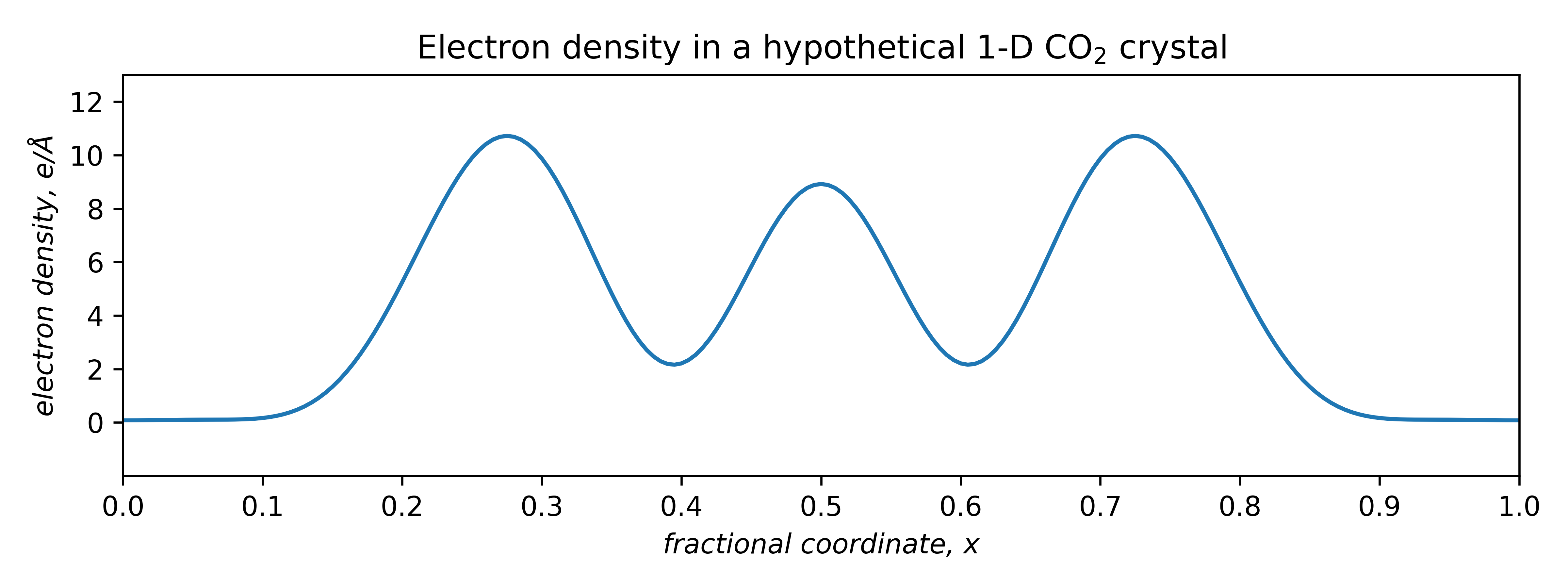
Before answering that, here's a quick review of some properties of sines and cosines:
Sine and cosine waves differ in phase by a quarter of a period (i.e., 90° or
π/2 radians). In crystallography it is more natural to use fractions of a period
than degrees or radians. The above plot shows that over one period, the cosine curve is
symmetric, while the sine is anti-symmetric, i.e.,
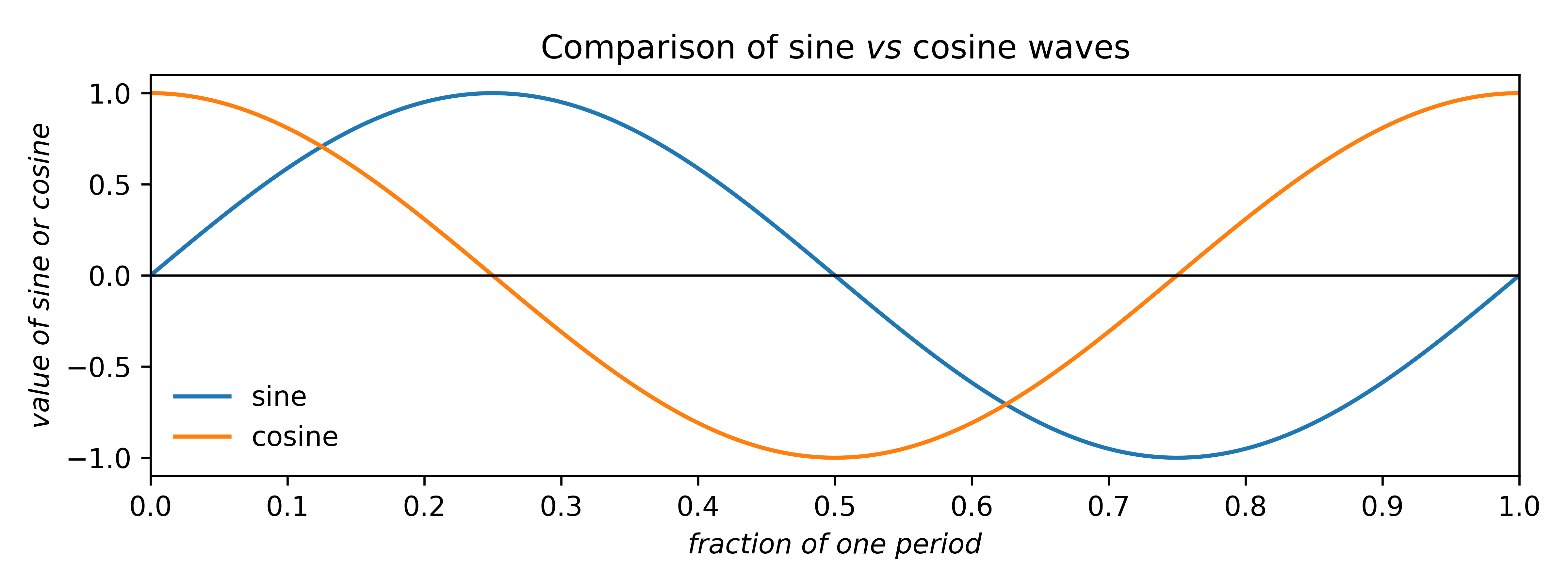
Since our example is centrosymmetric, the sine terms all cancel, so we can disregard them. For cosines, there are only two possible phases that preserve centrosymmetry: zero (as above) or shifted by half a period. The two possibilities are drawn below.
Since cosines range from –1 → +1, the area under either curve is zero. Such plots can be scaled by multiplying the cosine by a constant multiplier, or coefficient:
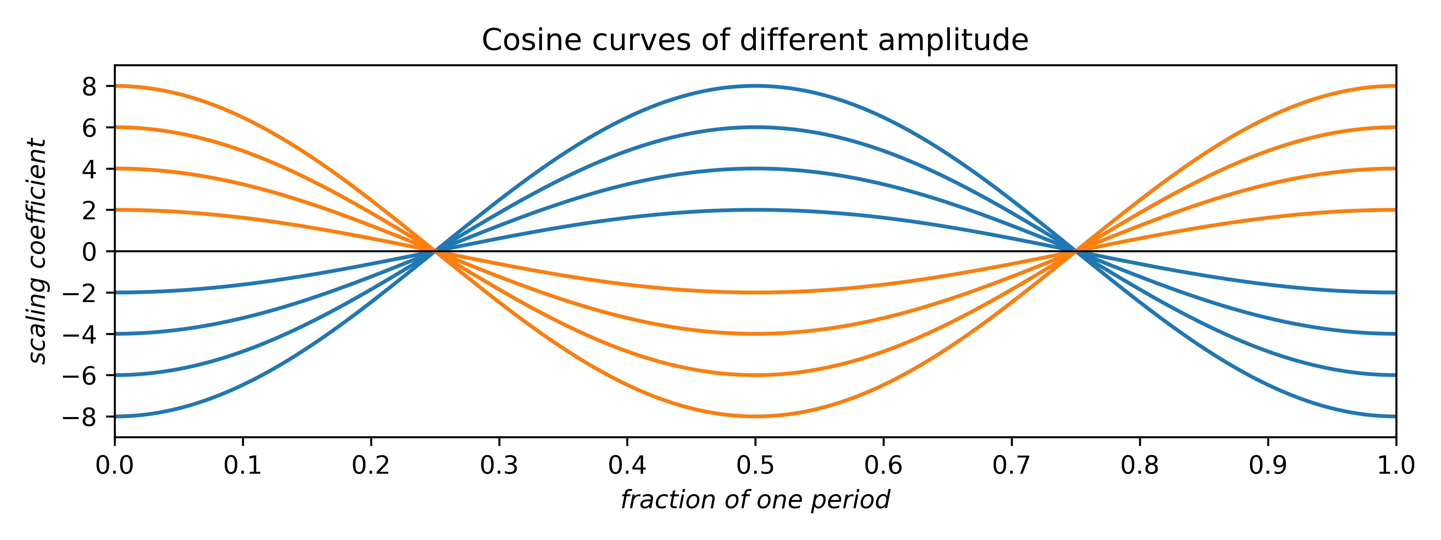
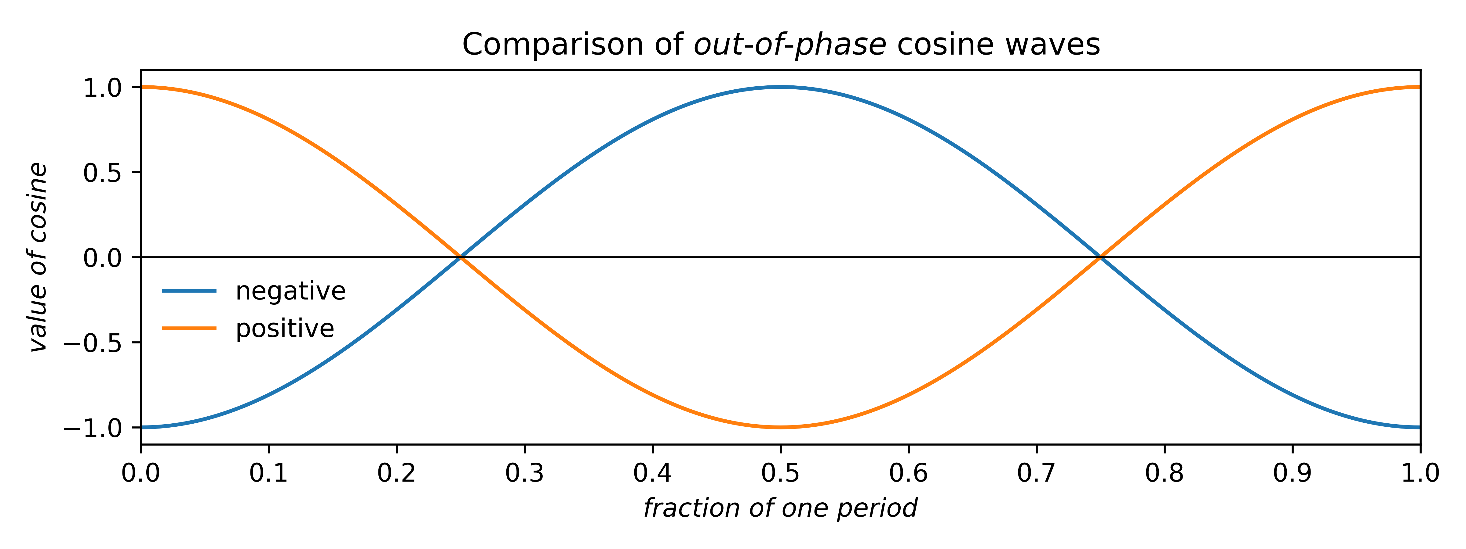
The coefficients can be any real number. Negative coefficients invert the plot and therefore have the effect of phase-shifting the wave by half a period. Thus, the two allowed phases (for centrosymmetry; non-centrosymmetry is more complicated) arise from waves having either positive or negative coefficients. In addition to amplitude and phase, cosine (and sine) waves can have different frequency:
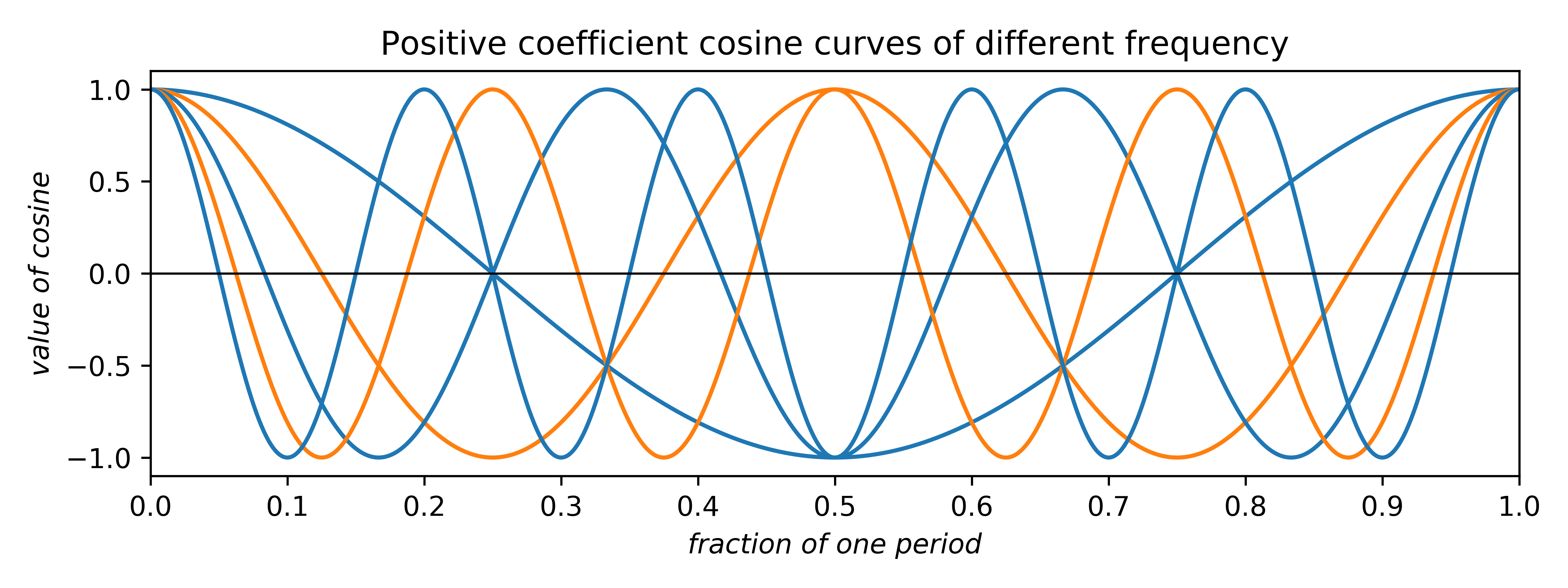
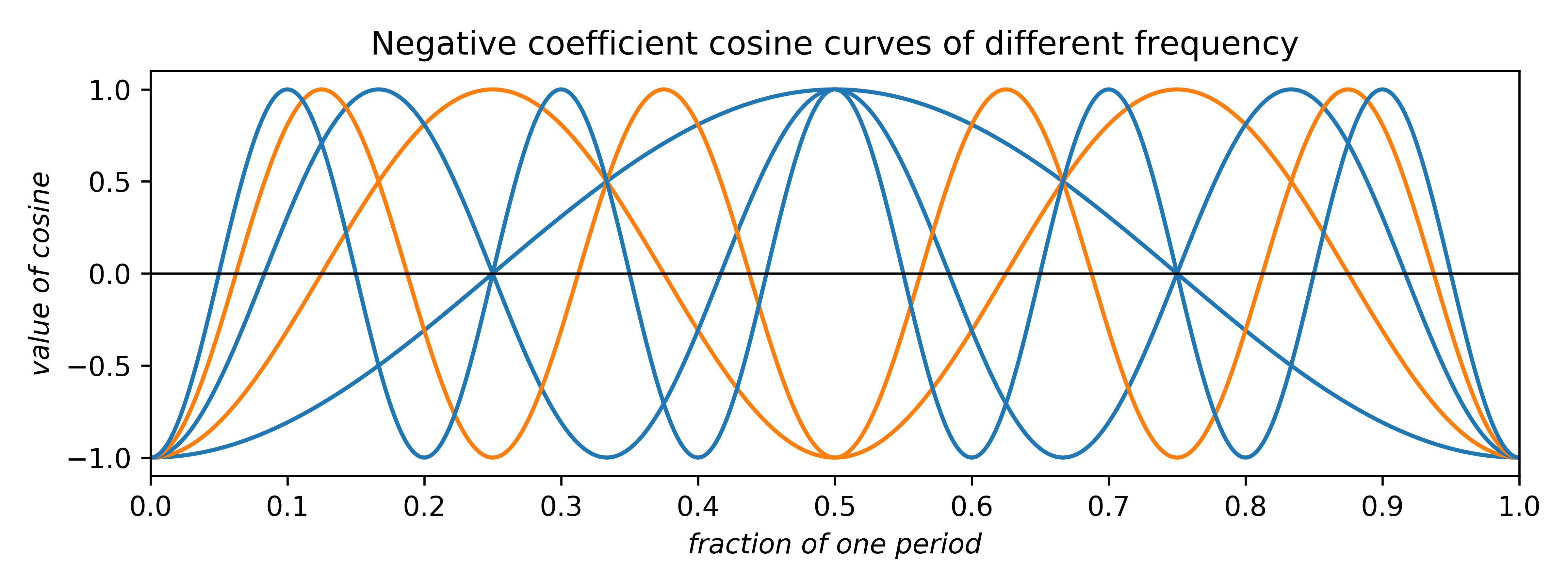
In the uppermost of the above two plots, positive-coefficient odd-frequency waves (blue) have minima at the centre and positive-coefficient even-frequency waves (orange) have maxima. In the lowermost plot for negative coefficients the situation is reversed.
Since our example is centrosymmetric, the anti-symmetric nature of the sine function, in our case
dictates that all the sine functions cancel, leaving
The term in the above summation for h = 0 is a special case because the cosine evaluates to exactly 1. Thus, the value for F (0) can be removed from the summation. This quantity, F (0) is simply the number of electrons in the unit cell. For a real crystal in 3D, this quantity is F (000). It is the amount needed to shift the electron density plot en masse upwards so that the electron count over the whole unit cell is correct. For one CO2 molecule, that's 22e–.
Lastly, due to the cosine function being symmetric, i.e.,
The summation need only cover the positive h indices, (or negative, or a unique unsigned combination thereof) viz.
for h = 1 to |hmax |
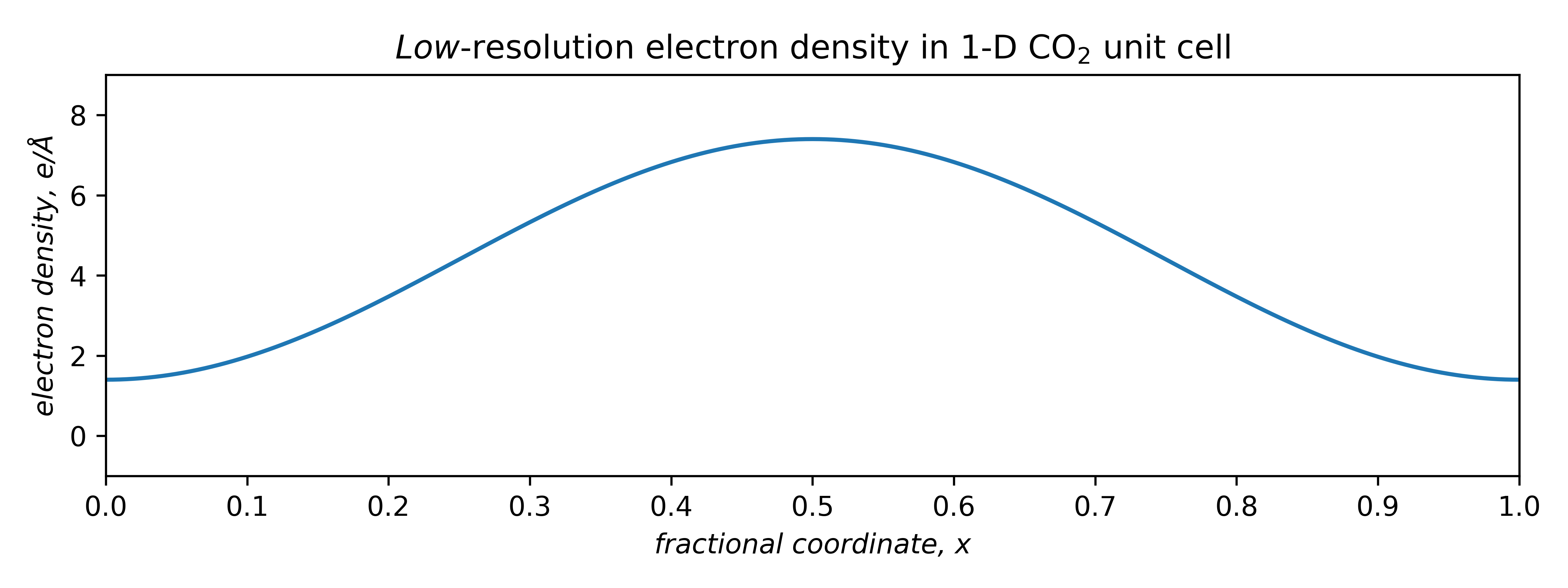
To model electron density, consider first the lowest-frequency term only. A negative coefficient, appropriately scaled and shifted upwards by F (0) to ensure an integral over the unit cell of 22e–, gives a very low-resolution electron density plot. It peaks in the middle of the cell, which happens to be where we placed the molecule:
A better fit requires more terms, each with its own frequency, amplitude, and phase (sign).
The next step is to identify the dominant frequencies and their amplitudes. These come from the Fourier transform of the actual electron density. The amplitudes, or Fourier coefficients, correspond to peak heights in the Fourier transform, as shown below:
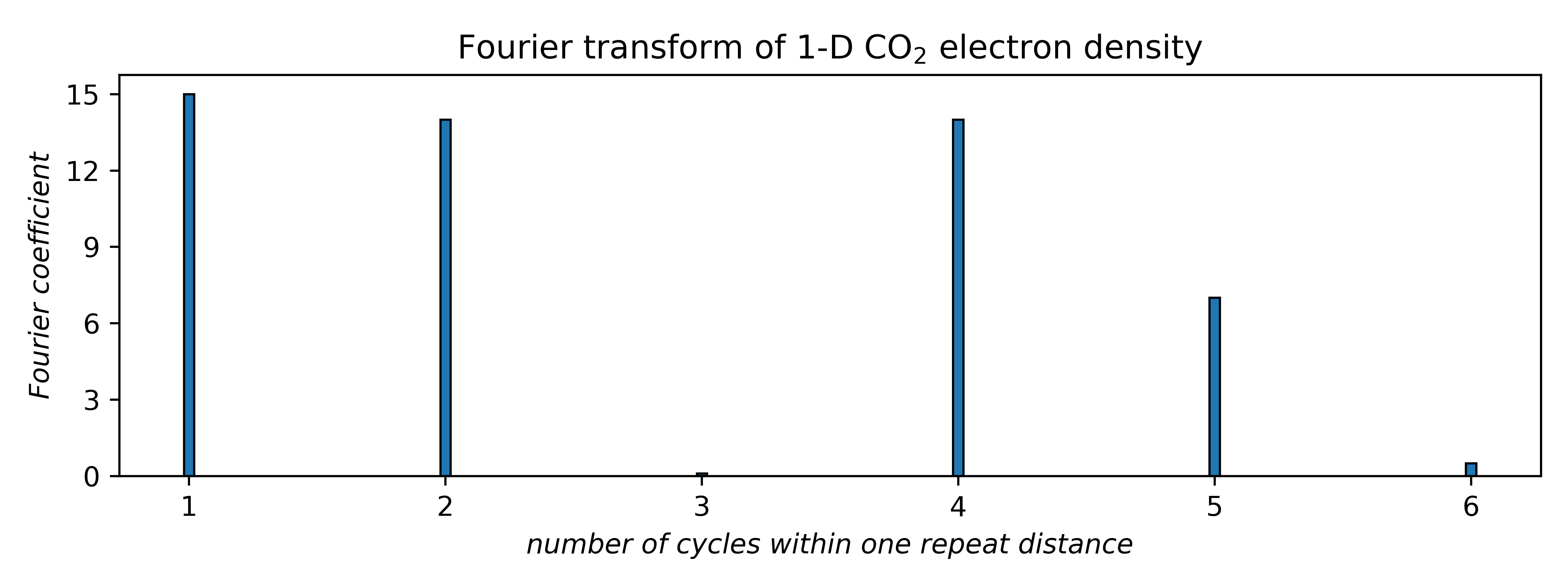
The connection to X-ray diffraction is that the Fourier coefficients are proportional to the square root of diffracted intensities. These are the structure factors, F (hkl ), in the first equation above. Here, the coefficients for frequencies 3 and 6 are tiny, so we'll ignore them (for now). That leaves four waves, each having a positive or negative coefficient, i.e., two possibilities apiece. Unfortunately, the Fourier transform gives no phase (sign) information. For four waves there are 24 = 16 different combinations, viz.
+ + – + – – + – + + – – – – + +
+ – + + – + – – + – + – – + – +
+ – – + – + + – + – – – – + + +
Since there are only 16 combinations, we can easily plot them all and compare:
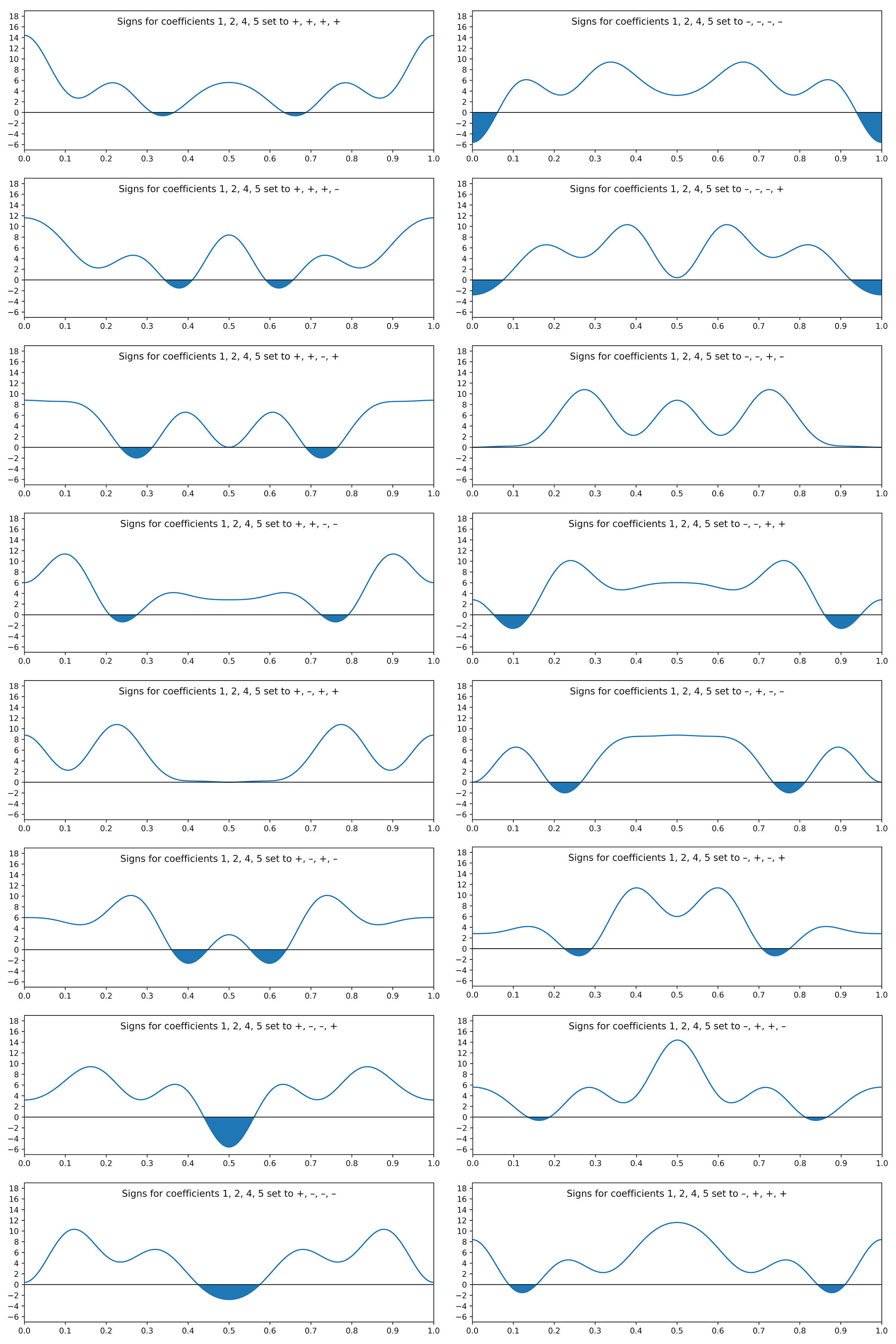
The shaded regions are negative and therefore cannot represent electron density. Thus, all but two of the sign combinations can be rejected. Note also that flipping all of the signs merely inverts the plot (prior to shifting it upwards to ensure an electron count of 22e–).
The two plots that are positive everywhere have "– – + –" and "+ – + +" sign combinations. These two plots are equivalent, but shifted relative to each other along x by half a unit cell repeat:
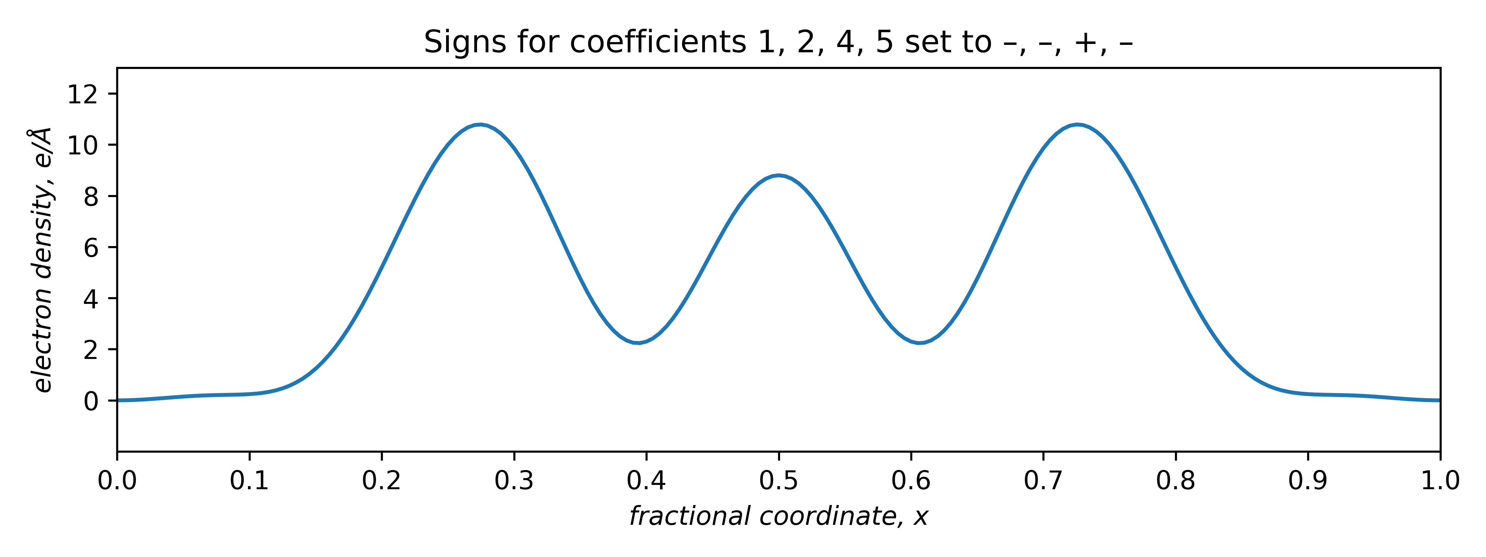
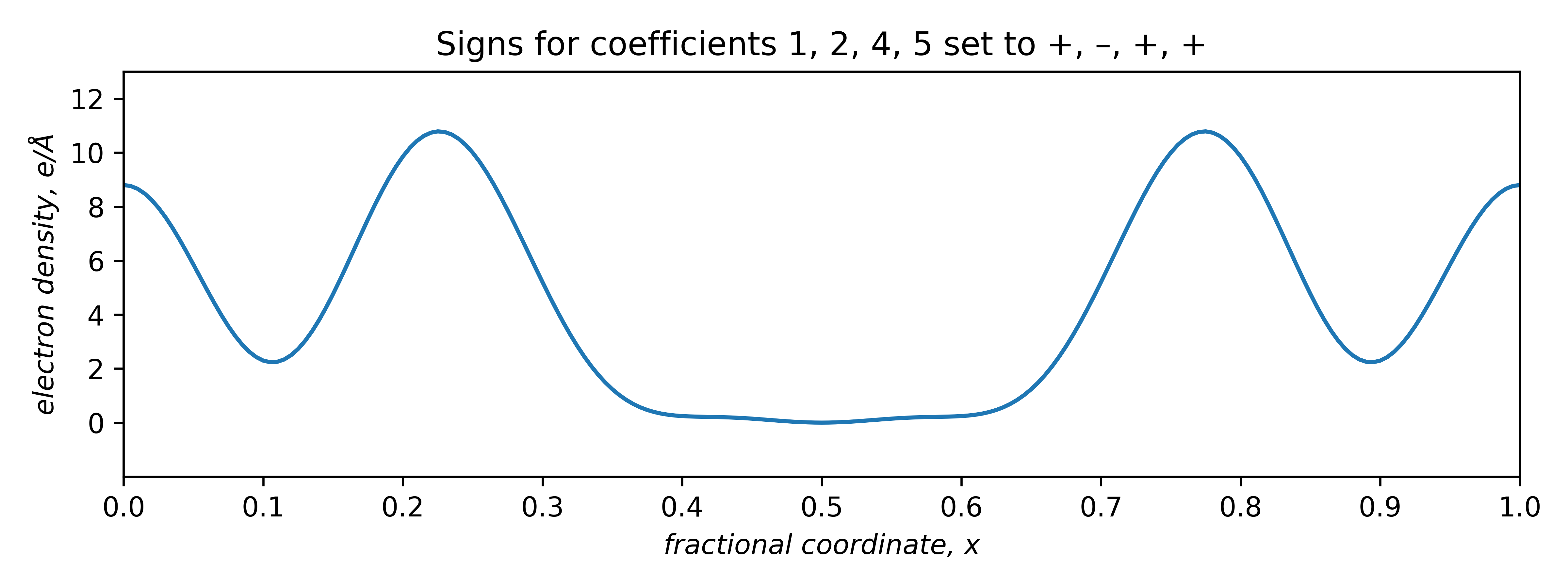
The signs of odd coefficients are flipped, while the even coefficient signs remain the same. The slight baseline ripple in the two plots above stem from ignoring the small coefficients of order 3 and 6 (and higher!). Setting the first coefficient as either negative or positive has the effect of fixing the origin. A real tri-periodic structure usually requires setting the signs of three (well-chosen) reflections.
Atom coordinates can be extracted directly from such plots:
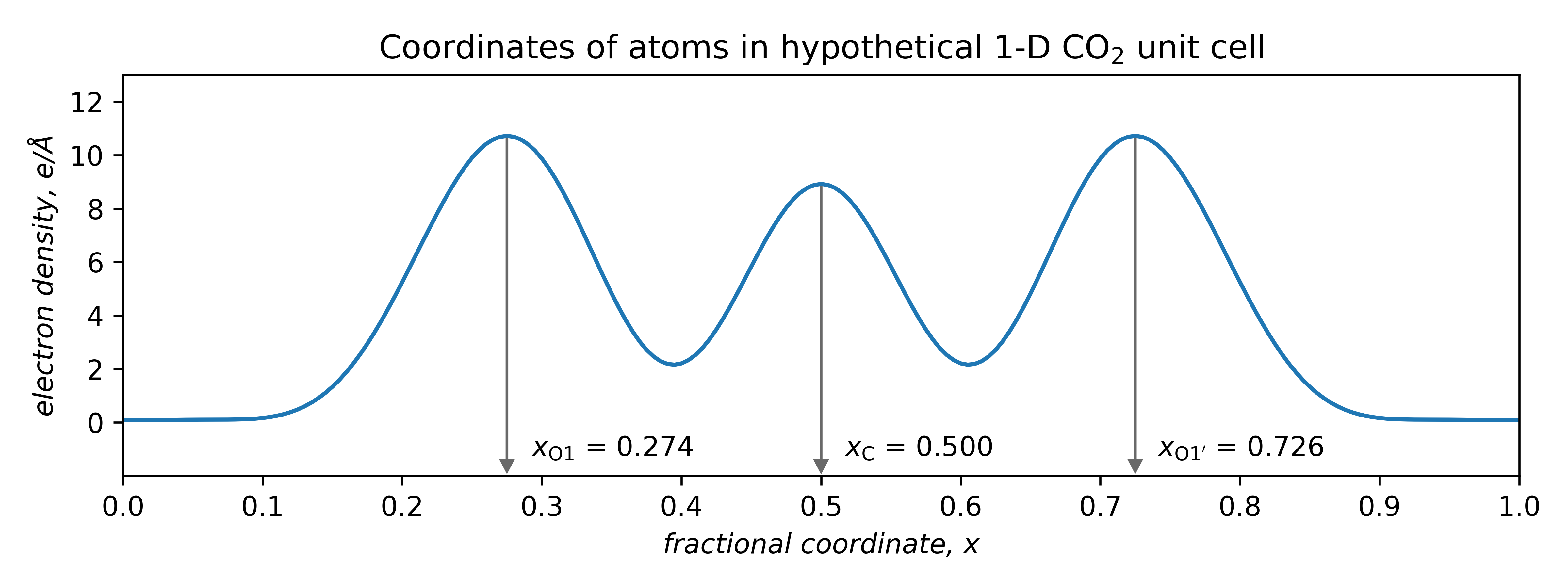
Thus, geometric parameters can be calculated. Here, the difference between carbon and either of the oxygen coordinates is 0.226. Since the unit cell length was 5.00 Å, the C—O interatomic distances (bond lengths) are:
For comparison, the actual bond length in CO2 is 1.16 Å. Not a bad result for a made-up analogy! Especially since in routine X-ray crystal structures, the accuracy of light atom positions is limited to about ±0.02 Å due to the way atomic scattering factors are approximated (the spherical atomic scattering factor approximation ).
Also apparent is that symmetry is of profound importance. This mono-periodic CO2 structure is symmetric by reflection through the points x = 0, 0.5, 1, etc. Atom O1' is equivalent to O1 by reflection through x = 0.5, viz.
Due to symmetry, only the region from x = 0 → 0.5 needs to be specified, thereby halving the computational burden. The smallest fragment needed to generate the whole structure is thus not the unit cell, but in this case, just half of it.
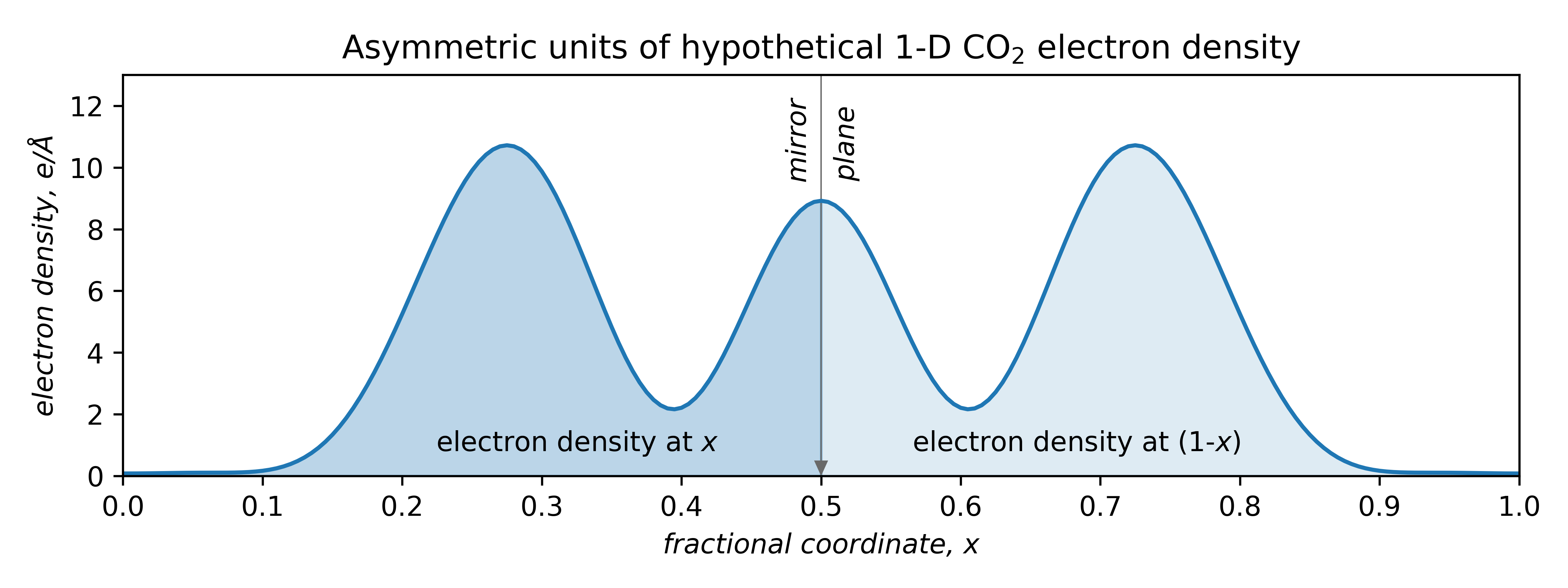
The unique part is the asymmetric unit : the fundamental building block of crystal structures. Different space groups have their own asymmetric units (details are in the International Tables, vol. A). Atoms on a point-symmetry element (x = 0, 0.5, 1 in the above) occupy a so-called special position. Atoms not on a special position occupy a general position.
For a real structure with thousands of diffraction maxima, the number of phase combinations is vast. A typical structure might result in ~5000 reflections, giving ~25000 sign combinations. A bit of quick log base conversion maths tells us that's ~101505. For comparison, the number of atoms in the known universe is ~1080. Clearly, we can't just guess the right phases! That is why the phase problem in crystallography is a problem.